Plotting statistically significant temperature trends with stippling

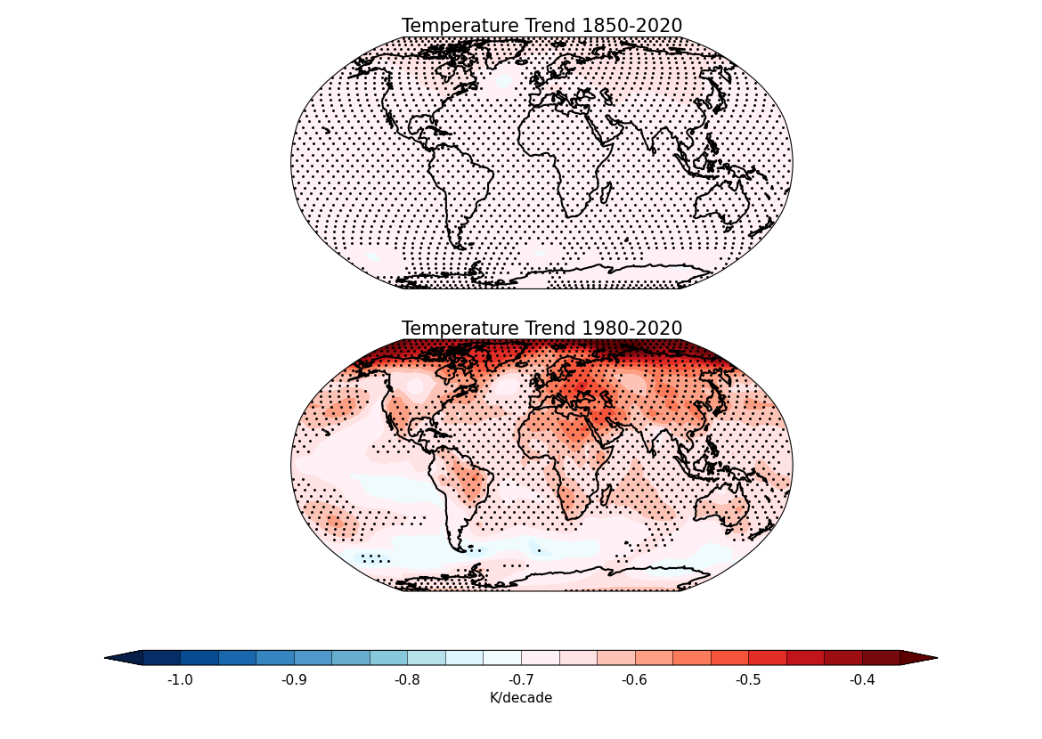
In this recipe, we will analyse and plot temperature trends from the HadCRUT.5.0.1.0 dataset for two different time periods. The plotted maps also include stippling, which is used to highlight areas where the temperature trends are statistically significant.

1. Import cf-python, cf-plot, numpy and scipy.stats:

import cfplot as cfp
import numpy as np
import scipy.stats as stats

import cf

2. Three functions are defined:

• linear_trend(data, time_axis): This function calculates the linear regression slope and p-value for the input data along the time axis. It takes two arguments: 'data', which represents the temperature anomalies or any other data you want to analyse, and 'time_axis', which represents the corresponding time points for the data. The function uses the stats.linregress method from the scipy.stats library to calculate the slope and p-value of the linear regression. It returns these two values as a tuple:

def linear_trend(data, time_axis):
    slope, _, _, p_value, _ = stats.linregress(time_axis, data)
    return slope, p_value

• create_trend_stipple_obj(temp_data, input_data): This function creates a new object with the input data provided and collapses the time dimension by taking the mean. It takes two arguments: 'temp_data', which represents the temperature data object, and 'input_data', which is the data to be set in the new object. The function creates a copy of the 'temp_data' object by selecting the first element using index and squeezes it to remove the size 1 axis. It then sets the input data with the 'Y' (latitude) and 'X' (longitude) axes, and then collapses the time dimension using the "T: mean" operation:

def create_trend_stipple_obj(temp_data, input_data):
    trend_stipple_obj = temp_data[0].squeeze()
    trend_stipple_obj.set_data(input_data, axes=["Y", "X"])
    return trend_stipple_obj

• process_subsets(subset_mask): This function processes the subsets of data by applying the linear_trend function along a specified axis. It takes one argument, 'subset_mask', which is a boolean mask representing the time points to be considered in the analysis. The function first extracts the masked subset of data and then applies the linear_trend function along the time axis (axis 0) using the numpy.ma.apply_along_axis function. The result is an array containing the slope and p-value for each grid point in the dataset:

def process_subsets(subset_mask):
    subset_data = masked_data[subset_mask, :, :]
    return np.ma.apply_along_axis(
        linear_trend, 0, subset_data, time_axis[subset_mask]
    )

3. Read the field constructs:

temperature_data = cf.read(
    "~/recipes/HadCRUT.5.0.1.0.analysis.anomalies.ensemble_mean.nc"
)[0]
print(temperature_data)

Field: long_name=blended air_temperature_anomaly over land with sea_water_temperature_anomaly (ncvar%tas_mean)
--------------------------------------------------------------------------------------------------------------
Data            : long_name=blended air_temperature_anomaly over land with sea_water_temperature_anomaly(time(2074), latitude(36), longitude(72)) K
Cell methods    : area: mean (interval: 5.0 degrees_north) time(2074): mean (interval: 1 month) realization(1): mean
Dimension coords: time(2074) = [1850-01-16 12:00:00, ..., 2022-10-16 12:00:00] gregorian
                : latitude(36) = [-87.5, ..., 87.5] degrees_north
                : longitude(72) = [-177.5, ..., 177.5] degrees_east
                : realization(1) = [100] 1

4. Calculate the annual mean temperature anomalies. The 'weights=True' argument is used take the varying lengths of months into account which ensures that the calculated mean is more accurate. A masked array is created for the annual mean temperature anomalies, masking any invalid values:

annual_temperature = temperature_data.collapse(
    "T: mean", weights=True, group=cf.Y()
)
time_axis = annual_temperature.coordinate("T").year.array
masked_data = np.ma.masked_invalid(annual_temperature.array)

5. Define two time periods for analysis: 1850-2020 and 1980-2020, along with a significance level (alpha) of 0.05:

time_periods = [(1850, 2020, "sub_1850_2020"), (1980, 2020, "sub_1980_2020")]
alpha = 0.05
results = {}

6. Loop through the time periods, processing the subsets, calculating trend p-values, and creating stipple objects. For each time period, the script calculates the trends and p-values using the process_subsets function. If the p-value is less than the significance level (alpha = 0.05), a stippling mask is created. The script then creates a new object for the trend and stippling mask using the create_trend_stipple_obj function:

for start, end, prefix in time_periods:
    subset_mask = (time_axis >= start) & (time_axis <= end)
    subset_trend_pvalue = process_subsets(subset_mask)
    results[prefix + "_trend_pvalue"] = subset_trend_pvalue
    results[prefix + "_stipple"] = subset_trend_pvalue[1] < alpha
    results[prefix + "_trend"] = create_trend_stipple_obj(
        temperature_data, subset_trend_pvalue[0]
    )
    results[prefix + "_stipple_obj"] = create_trend_stipple_obj(
        temperature_data, results[prefix + "_stipple"]
    )

7. Create two plots - one for the 1850-2020 time period and another for the 1980-2020 time period using cfplot.con. The results are multiplied by 10 so that each plot displays the temperature trend in K/decade with stippling to indicate areas where the trend is statistically significant (p-value < 0.05). Here cfplot.gopen is used to define the parts of the plot area with two rows and one column, and setting the bottom margin to 0.2. It is closed by cfplot.gclose; cfplot.gpos is used to set the plotting position of both the plots; cfplot.mapset is used to set the map projection to Robinson; cfplot.cscale is used to choose one of the colour maps amongst many available; cfplot.levs is used to set the contour levels; and cfplot.stipple is used to add stippling to show statistically significant areas:

cfp.gopen(rows=2, columns=1, bottom=0.2)

cfp.gpos(1)
cfp.mapset(proj="robin")
cfp.cscale("temp_19lev")
cfp.levs(min=-1, max=1, step=0.1)
cfp.con(
    results["sub_1850_2020_trend"] * 10,
    lines=False,
    colorbar=None,
    title="Temperature Trend 1850-2020",
)
cfp.stipple(
    results["sub_1850_2020_stipple_obj"],
    min=1,
    max=1,
    size=5,
    color="k",
    marker=".",
)

cfp.gpos(2)
cfp.mapset(proj="robin")
cfp.cscale("temp_19lev")
cfp.levs(min=-1, max=1, step=0.1)
cfp.con(
    results["sub_1980_2020_trend"] * 10,
    lines=False,
    title="Temperature Trend 1980-2020",
    colorbar_position=[0.1, 0.1, 0.8, 0.02],
    colorbar_orientation="horizontal",
    colorbar_title="K/decade",
)
cfp.stipple(
    results["sub_1980_2020_stipple_obj"],
    min=1,
    max=1,
    size=5,
    color="k",
    marker=".",
)

cfp.gclose()

Warning - boolean data found - converting to integers






Warning - boolean data found - converting to integers