Transformation/interpolation interface
Clicking on the Trans button in the main xconv window brings up the Transformation/Interpolation interface.
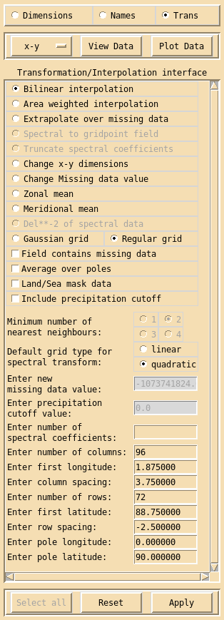
The Transformation/Interpolation interface can be used to modify both spectral and grid point data. This interface only sets the variables needed to modify the data, the actual transformation/interpolation is done when the data is either viewed, plotted or written out. Only sections which are relevant to the current field and configuration will be usable the others will be inactive. The Transformation/Interpolation interface can be applied successively to the same field.
If data is in the form of spectral coefficients and needs to be converted to a grid point format then select Spectral to gridpoint field. There are various options available to define the new grid. Two grid types can be selected either a Gaussian grid or a regular grid. If the data is to be transformed to the grid equivalent of a particular spectral truncation then select either a linear or quadratic grid type, enter the number of spectral coefficients and press return. This will then automatically fill in the correct x and y grid parameters. Alternatively enter the number of columns (nlong) and press return, this will assume the first longitude is at 0 and fill in the correct column spacing for a global grid. Similarly enter the number of rows (nlat) and press return, this will fill in the correct first latitude and row spacing for a global grid which does not pass though the equator. If a different grid definition is needed then all the relevant boxes must be filled in. For a Gaussian grid only the number of rows is needed for the latitude dimension. Spectral coefficients must be transformed to a global grid, but you can use a two step method to transform to a limited area grid. For example you could convert T106 spectral data to a Unified model limited area grid using the following method: Transform the T106 spectral data to a 320x160 Gaussian grid, click on the Apply button, you now have a grid point field which you can interpolate onto a regular limited area grid with a rotated pole, see below.
If Truncate spectral coefficients is selected then the new number of spectral coefficients must be entered. The truncation is done be chopping off the higher wave numbers, or if a number larger than current number of spectral coefficients is entered then the existing coefficients are padded out with zeros.
To apply a inverse Laplacian operator to spectral data select Del**-2 of spectral data. This will convert vorticity into stream function and divergence into velocity potential.
Grid point data can be interpolated onto a new grid, either using Bilinear interpolation or Area weighted interpolation, the new grid is defined in exactly the same way as above for spectral transformations. There are extra options available for grid point interpolation. If a field contains missing data values, then the relevant button should be selected, this will prevent xconv from using missing data values as real data values. If this option is selected and the field does not contain missing data values the field is still interpolated correctly but it will take slightly longer to do. If Average over poles is selected then xconv will replace the polar values with an average value, if the interpolated data does not contain polar values then this option will have no effect. If the data is a Land/Sea mask, or any data which consists entirely of 0’s and 1’s (or 0’s and -1’s), then option Land/Sea mask data should be selected. The use of bilinear interpolation can result in fields being smeared over the output grid. It is recognised that this may not be appropriate for precipitation type fields, and xconv includes an option to remove all interpolated precipitation at grid boxes where the interpolated value is less than a user-defined cutoff value. If this option is required then Include precipitation cutoff should selected and a value for the precipitation cutoff should be entered. The precipitation cutoff is implemented in two steps, firstly any output field value less than the cutoff value will be set to zero. Secondly, for each output grid point, the nearest input field grid point is determined, if the value of precipitation at this latter point in the input data field is less than the cutoff value, then the precipitation at the output grid point is set to zero. The area weighted interpolation option does not allow fields with missing data to be handled differently or for a precipitation cutoff to be used. It is possible to interpolate onto a grid with a rotated pole, such as the limited area grids used in the Met. Office Unified Model. To do this the longitude and latitude of the rotated north pole must be entered.
If the grid point data contains missing data the option Extrapolate over missing data will replace missing data values using nearest neighbour filling. The minimum number of nearest neighbours should be selected (1,2,3 or 4), the default value is 2. This option can be useful when, for example, interpolating SST data (with missing data over land points) onto a new grid. In this case care must be taken that a missing data value on the original grid is not mapped onto a real data value on the new grid. If the extrapolate option is used to replace missing data before the interpolation step, this problem will not happen.
Another option for grid point fields is Change x-y dimensions, this allows you to change the values of the x and y dimensions but not the number of rows or columns. This option only changes the dimension values, the data values are unaffected. This option can be useful when you have data from different sources on essentially the same grid, except for slight differences due to, for example, rounding error. If you wanted to difference this data some utilities will complain that the data is on different grids, using this option you can force the x and y dimension values to be the same.
If there was an error when creating the data and the missing data indicator does not agree with the actual missing data values used then the Change Missing data value option can be useful. If the correct value of the missing data is entered then when the data is converted the error in the missing data indicator will be fixed.
Finally for grid point fields you can do a Zonal mean or a Meridional mean.
The Apply button must be clicked for any transformation or interpolation changes to take effect. The Reset button will reset the transformation or interpolation information to either its initial state if Apply has not yet been used or to the state it was in when Apply was last used.