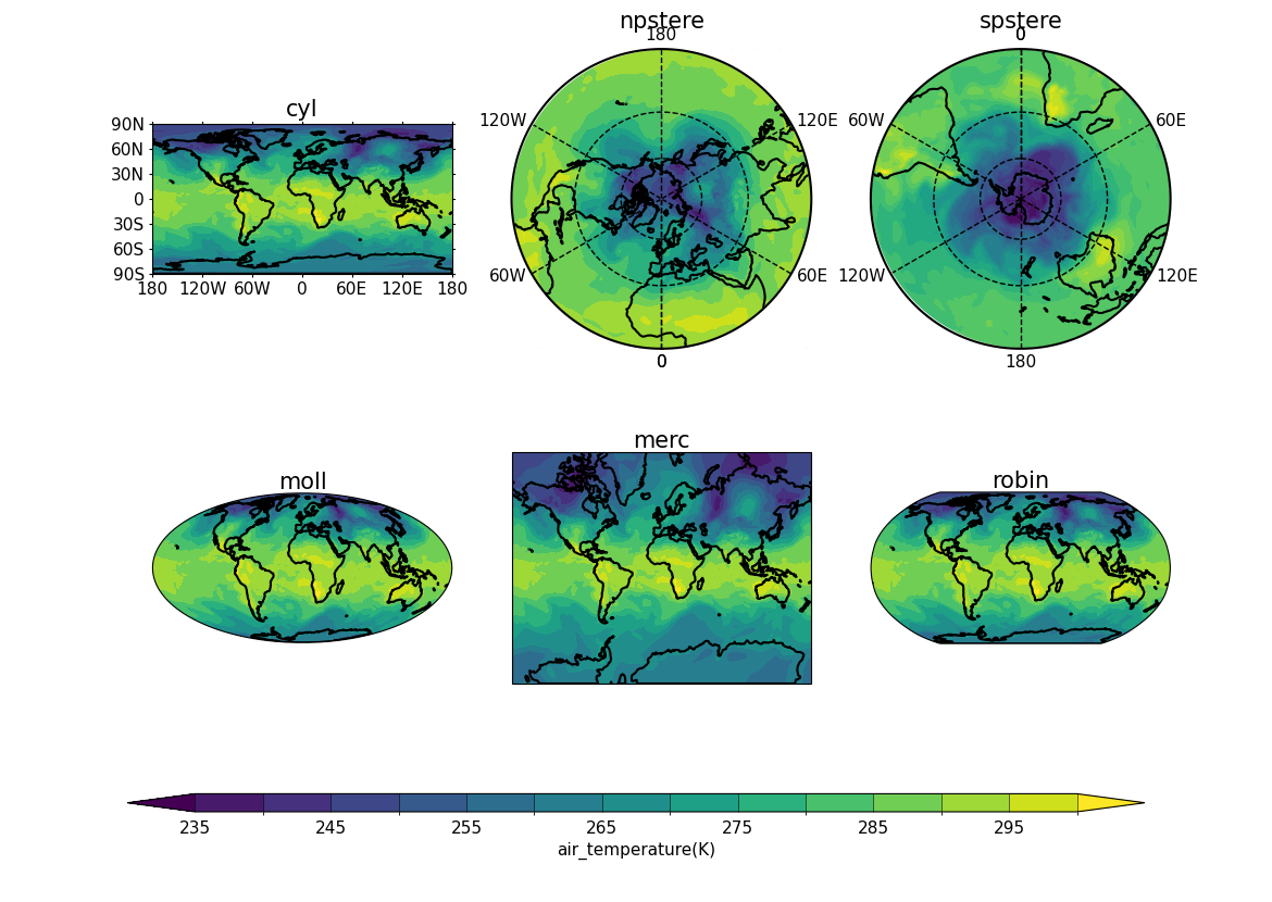
Plotting contour subplots with different projections

In this recipe, we will plot the same data using different projections as subplots to illustrate visually some available possibilities.

1. Import cf-python and cf-plot:

import cfplot as cfp

import cf

2. Read the field in:

f = cf.read("~/recipes/ggap.nc")[0]

3. List the projection types to use. Here we are using Cylindrical/Default, North Pole Stereographic, South Pole Stereographic, Mollweide, Mercator and Robinson. However there are several other choices possible, see: https://ncas-cms.github.io/cf-plot/build/user_guide.html#appendixc. Our chosen list is:

projtypes = ["cyl", "npstere", "spstere", "moll", "merc", "robin"]

4. Create the file with subplots. If changing the number of subplots, ensure the number of rows * number of columns = the number of projections. Here we are doing 6 projections so 2 x 3 is fine. Then loop through the list of projection types and plot each as a sub-plot:

cfp.gopen(rows=2, columns=3, bottom=0.2)
for i, proj in enumerate(projtypes):
    # gpos has 1 added to the index because it takes 1 as its first value
    cfp.gpos(i + 1)
    cfp.mapset(proj=proj)

    # For the final plot only, add a colour bar to cover all the sub-plots
    if i == len(projtypes) - 1:
        cfp.con(
            f.subspace(pressure=850),
            lines=False,
            title=proj,
            colorbar_position=[0.1, 0.1, 0.8, 0.02],
            colorbar_orientation="horizontal",
        )
    else:
        cfp.con(
            f.subspace(pressure=850),
            lines=False,
            title=proj,
            colorbar=False,
        )
cfp.gclose()