Tutorial
Version 3.20.1 for version 1.13 of the CF conventions.
All of the Python code in this tutorial is available in two executable
scripts (download, 28kB,
download, 8kB).
Sample datasets
This tutorial uses a number of small sample datasets, all of which can
be found in the zip file cf_tutorial_files.zip
(download,
164kB):
$ unzip -q cf_tutorial_files.zip
$ ls -1
air_temperature.nc
cf_tutorial_files.zip
contiguous.nc
external.nc
file2.nc
file.nc
gathered.nc
parent.nc
precipitation_flux.nc
timeseries.nc
umfile.pp
vertical.nc
wind_components.nc
The tutorial examples assume that the Python session is being run from the directory that contains the zip file and its unpacked contents, and no other files.
The tutorial files may be also found in the downloads directory of the on-line code repository.
Import
The cf package is imported as follows:
>>> import cf
Tip
It is possible to change the extent to which cf outputs feedback messages and it may be instructive to increase the verbosity whilst working through this tutorial to see and learn more about what cf is doing under the hood and about the nature of the dataset being operated on. See the section on ‘Logging’ for more information.
CF version
The version of the CF conventions and
the CF data model being used may be found with
the cf.CF function:
>>> cf.CF()
'1.8'
This indicates which version of the CF conventions are represented by this release of the cf package, and therefore the version can not be changed.
Note, however, that datasets of different CF versions may be read from, or written to netCDF.
Field and domain constructs
The central constructs of CF are the field construct and domain construct.
The field construct, that corresponds to a CF-netCDF data variable, includes all of the metadata to describe it:
descriptive properties that apply to field construct as a whole (e.g. the standard name),
a data array, and
“metadata constructs” that describe the locations of each cell (i.e. the “domain”) of the data array, and the physical nature of each cell’s datum.
Likewise, the domain construct, that corresponds to a CF-netCDF domain variable or to the domain of a field construct, includes all of the metadata to describe it:
descriptive properties that apply to field construct as a whole (e.g. the long name), and
metadata constructs that describe the locations of each cell of the domain.
A field construct or domain construct is stored in a cf.Field
instance or cf.Domain instance respectively. Henceforth the phrase
“field construct” will be assumed to mean “cf.Field instance”, and
“domain construct” will be assumed to mean “cf.Domain instance”.
Reading field constructs from datasets
The cf.read function reads files from disk, or from an OPeNDAP URLs [1], and returns the contents in
a cf.FieldList instance that contains zero or more field constructs.
A field list is very much like a Python list,
with the addition of extra methods that operate on its field construct
elements.
The following file types can be read:
All formats of netCDF3 and netCDF4 files can be read, containing datasets for any version of CF up to and including CF-1.13, including UGRID datasets.
Files in CDL format, with or without the data array values.
Datasets in Zarr v2 (xarray-style) and Zarr v3 formats.
Datasets in Kerchunk format.
PP and UM fields files, whose contents are mapped into field constructs.
Note that when reading netCDF4 files that contain hierachical groups, the group structure is saved via the netCDF interface so that it may be re-used, or modified, if the field constructs are written to back to disk.
For example, to read the file file.nc (found in the sample
datasets), which contains
two field constructs:
>>> x = cf.read('file.nc')
>>> type(x)
<class 'cf.fieldlist.FieldList'>
>>> len(x)
2
Descriptive properties are always read into memory, but lazy loading is employed for all data arrays, which means that no data is read into memory until the data is required for inspection or to modify the array contents. This maximises the number of field constructs that may be read within a session, and makes the read operation fast.
Multiple files may be read in one command using UNIX wild card characters, or a sequence of file names (each element of which may also contain wild cards). Shell environment variables are also permitted.
>>> y = cf.read('*.nc')
>>> len(y)
14
>>> z = cf.read(['file.nc', 'precipitation_flux.nc'])
>>> len(z)
3
All of the datasets in one or more directories may also be read by replacing any file name with a directory name. An attempt will be made to read all files in the directory, which will result in an error if any have a non-supported format. Non-supported files may be ignored by being more specific about the file type intended for reading in using the dataset_type keyword:
>>> y = cf.read('$PWD')  # Raises Exception
Traceback (most recent call last):
    ...
Exception: Can't determine format of file cf_tutorial_files.zip
>>> y = cf.read('$PWD', dataset_type='netCDF')
>>> len(y)
15
In all cases, the default behaviour is to aggregate the contents of
all input datasets into as few field constructs as possible, and it is
these aggregated field constructs are returned by cf.read. See the
section on aggregation for full details.
The cf.read function has optional parameters to
allow the user to provide files that contain external variables;
request extra field constructs to be created from “metadata” netCDF variables, i.e. those that are referenced from CF-netCDF data variables, but which are not regarded by default as data variables in their own right;
return only domain constructs derived from CF-netCDF domain variables;
request that masking is not applied by convention to data elements (see data masking);
issue warnings when
valid_min,valid_maxandvalid_rangeattributes are present (see data masking);display information and issue warnings about the mapping of the netCDF file contents to CF data model constructs;
remove from, or include, size one dimensions on the field constructs’ data;
configure the field construct aggregation process;
configure the reading of directories to allow sub-directories to be read recursively, and to allow directories which resolve to symbolic links; and
choose either
netCDF4orh5netcdfbackends for accessing netCDF files.configure parameters for reading PP and UM fields files.
CF-compliance
If the dataset is partially CF-compliant to the extent that it is not
possible to unambiguously map an element of the netCDF dataset to an
element of the CF data model, then a field construct is still
returned, but may be incomplete. This is so that datasets which are
partially conformant may nonetheless be modified in memory and written
to new datasets. Such “structural” non-compliance would occur, for
example, if the coordinates attribute of a CF-netCDF data variable
refers to another variable that does not exist, or refers to a
variable that spans a netCDF dimension that does not apply to the data
variable. Other types of non-compliance are not checked, such whether
or not controlled vocabularies have been adhered to. The structural
compliance of the dataset may be checked with the
dataset_compliance method of the field construct, as well
as optionally displayed when the dataset is read.
Inspection
The contents of a field construct may be inspected at three different levels of detail.
Minimal detail
The built-in repr function, invoked on a variable by calling that variable
alone at the interpreter prompt, returns a short, one-line description:
>>> x = cf.read('file.nc')
>>> x
[<CF Field: specific_humidity(latitude(5), longitude(8)) 1>,
 <CF Field: air_temperature(atmosphere_hybrid_height_coordinate(1), grid_latitude(10), grid_longitude(9)) K>]
>>> q = x[0]
>>> t = x[1]
>>> q
<CF Field: specific_humidity(latitude(5), longitude(8)) 1>
This gives the identity of the field construct (e.g. “specific_humidity”), the identities and sizes of the dimensions spanned by the data array (“latitude” and “longitude” with sizes 5 and 8 respectively) and the units of the data (“1”, i.e. dimensionless).
Medium detail
The built-in str function, invoked by a print call on a field construct,
returns similar information as the one-line output, along with short
descriptions of the metadata constructs, which include the first and last
values of their data arrays:
>>> print(q)
Field: specific_humidity (ncvar%q)
----------------------------------
Data            : specific_humidity(latitude(5), longitude(8)) 1
Cell methods    : area: mean
Dimension coords: latitude(5) = [-75.0, ..., 75.0] degrees_north
                : longitude(8) = [22.5, ..., 337.5] degrees_east
                : time(1) = [2019-01-01 00:00:00]
>>> print(t)
Field: air_temperature (ncvar%ta)
---------------------------------
Data            : air_temperature(atmosphere_hybrid_height_coordinate(1), grid_latitude(10), grid_longitude(9)) K
Cell methods    : grid_latitude(10): grid_longitude(9): mean where land (interval: 0.1 degrees) time(1): maximum
Field ancils    : air_temperature standard_error(grid_latitude(10), grid_longitude(9)) = [[0.76, ..., 0.32]] K
Dimension coords: atmosphere_hybrid_height_coordinate(1) = [1.5]
                : grid_latitude(10) = [2.2, ..., -1.76] degrees
                : grid_longitude(9) = [-4.7, ..., -1.18] degrees
                : time(1) = [2019-01-01 00:00:00]
Auxiliary coords: latitude(grid_latitude(10), grid_longitude(9)) = [[53.941, ..., 50.225]] degrees_N
                : longitude(grid_longitude(9), grid_latitude(10)) = [[2.004, ..., 8.156]] degrees_E
                : long_name=Grid latitude name(grid_latitude(10)) = [--, ..., b'kappa']
Cell measures   : measure:area(grid_longitude(9), grid_latitude(10)) = [[2391.9657, ..., 2392.6009]] km2
Coord references: grid_mapping_name:rotated_latitude_longitude
                : standard_name:atmosphere_hybrid_height_coordinate
Domain ancils   : ncvar%a(atmosphere_hybrid_height_coordinate(1)) = [10.0] m
                : ncvar%b(atmosphere_hybrid_height_coordinate(1)) = [20.0]
                : surface_altitude(grid_latitude(10), grid_longitude(9)) = [[0.0, ..., 270.0]] m
Note that time values are converted to date-times with the cftime package.
Full detail
The dump method of the field construct gives all
properties of all constructs, including metadata constructs and their
components, and shows the first and last values of all data arrays:
>>> q.dump()
----------------------------------
Field: specific_humidity (ncvar%q)
----------------------------------
Conventions = 'CF-1.11'
project = 'research'
standard_name = 'specific_humidity'
units = '1'

Data(latitude(5), longitude(8)) = [[0.003, ..., 0.032]] 1

Cell Method: area: mean

Domain Axis: latitude(5)
Domain Axis: longitude(8)
Domain Axis: time(1)

Dimension coordinate: latitude
    standard_name = 'latitude'
    units = 'degrees_north'
    Data(latitude(5)) = [-75.0, ..., 75.0] degrees_north
    Bounds:Data(latitude(5), 2) = [[-90.0, ..., 90.0]]

Dimension coordinate: longitude
    standard_name = 'longitude'
    units = 'degrees_east'
    Data(longitude(8)) = [22.5, ..., 337.5] degrees_east
    Bounds:Data(longitude(8), 2) = [[0.0, ..., 360.0]]

Dimension coordinate: time
    standard_name = 'time'
    units = 'days since 2018-12-01'
    Data(time(1)) = [2019-01-01 00:00:00]

>>> t.dump()
---------------------------------
Field: air_temperature (ncvar%ta)
---------------------------------
Conventions = 'CF-1.11'
project = 'research'
standard_name = 'air_temperature'
units = 'K'

Data(atmosphere_hybrid_height_coordinate(1), grid_latitude(10), grid_longitude(9)) = [[[0.0, ..., 89.0]]] K

Cell Method: grid_latitude(10): grid_longitude(9): mean where land (interval: 0.1 degrees)
Cell Method: time(1): maximum

Field Ancillary: air_temperature standard_error
    standard_name = 'air_temperature standard_error'
    units = 'K'
    Data(grid_latitude(10), grid_longitude(9)) = [[0.76, ..., 0.32]] K

Domain Axis: atmosphere_hybrid_height_coordinate(1)
Domain Axis: grid_latitude(10)
Domain Axis: grid_longitude(9)
Domain Axis: time(1)

Dimension coordinate: atmosphere_hybrid_height_coordinate
    computed_standard_name = 'altitude'
    standard_name = 'atmosphere_hybrid_height_coordinate'
    Data(atmosphere_hybrid_height_coordinate(1)) = [1.5]
    Bounds:Data(atmosphere_hybrid_height_coordinate(1), 2) = [[1.0, 2.0]]

Dimension coordinate: grid_latitude
    standard_name = 'grid_latitude'
    units = 'degrees'
    Data(grid_latitude(10)) = [2.2, ..., -1.76] degrees
    Bounds:Data(grid_latitude(10), 2) = [[2.42, ..., -1.98]]

Dimension coordinate: grid_longitude
    standard_name = 'grid_longitude'
    units = 'degrees'
    Data(grid_longitude(9)) = [-4.7, ..., -1.18] degrees
    Bounds:Data(grid_longitude(9), 2) = [[-4.92, ..., -0.96]]

Dimension coordinate: time
    standard_name = 'time'
    units = 'days since 2018-12-01'
    Data(time(1)) = [2019-01-01 00:00:00]

Auxiliary coordinate: latitude
    standard_name = 'latitude'
    units = 'degrees_N'
    Data(grid_latitude(10), grid_longitude(9)) = [[53.941, ..., 50.225]] degrees_N

Auxiliary coordinate: longitude
    standard_name = 'longitude'
    units = 'degrees_E'
    Data(grid_longitude(9), grid_latitude(10)) = [[2.004, ..., 8.156]] degrees_E

Auxiliary coordinate: long_name=Grid latitude name
    long_name = 'Grid latitude name'
    Data(grid_latitude(10)) = [--, ..., 'kappa']

Domain ancillary: ncvar%a
    units = 'm'
    Data(atmosphere_hybrid_height_coordinate(1)) = [10.0] m
    Bounds:Data(atmosphere_hybrid_height_coordinate(1), 2) = [[5.0, 15.0]]

Domain ancillary: ncvar%b
    Data(atmosphere_hybrid_height_coordinate(1)) = [20.0]
    Bounds:Data(atmosphere_hybrid_height_coordinate(1), 2) = [[14.0, 26.0]]

Domain ancillary: surface_altitude
    standard_name = 'surface_altitude'
    units = 'm'
    Data(grid_latitude(10), grid_longitude(9)) = [[0.0, ..., 270.0]] m

Coordinate reference: atmosphere_hybrid_height_coordinate
    Coordinate conversion:computed_standard_name = altitude
    Coordinate conversion:standard_name = atmosphere_hybrid_height_coordinate
    Coordinate conversion:a = Domain Ancillary: ncvar%a
    Coordinate conversion:b = Domain Ancillary: ncvar%b
    Coordinate conversion:orog = Domain Ancillary: surface_altitude
    Datum:earth_radius = 6371007
    Dimension Coordinate: atmosphere_hybrid_height_coordinate

Coordinate reference: rotated_latitude_longitude
    Coordinate conversion:grid_mapping_name = rotated_latitude_longitude
    Coordinate conversion:grid_north_pole_latitude = 38.0
    Coordinate conversion:grid_north_pole_longitude = 190.0
    Datum:earth_radius = 6371007
    Dimension Coordinate: grid_longitude
    Dimension Coordinate: grid_latitude
    Auxiliary Coordinate: longitude
    Auxiliary Coordinate: latitude

Cell measure: measure:area
    units = 'km2'
    Data(grid_longitude(9), grid_latitude(10)) = [[2391.9657, ..., 2392.6009]] km2
File inspection with cfa
The description for every field constructs found in datasets also be
generated from the command line, with minimal, medium or full detail,
by using the cfa tool, for example:
$ cfa file.nc
CF Field: air_temperature(atmosphere_hybrid_height_coordinate(1), grid_latitude(10), grid_longitude(9)) K
CF Field: specific_humidity(latitude(5), longitude(8)) 1
$ cfa -1 *.nc
CF Field: specific_humidity(cf_role=timeseries_id(4), ncdim%timeseries(9))
CF Field: cell_area(ncdim%longitude(9), ncdim%latitude(10)) m2
CF Field: eastward_wind(latitude(10), longitude(9)) m s-1
CF Field: specific_humidity(latitude(5), longitude(8)) 1
CF Field: air_potential_temperature(time(120), latitude(5), longitude(8)) K
CF Field: precipitation_flux(time(1), latitude(64), longitude(128)) kg m-2 day-1
CF Field: precipitation_flux(time(2), latitude(4), longitude(5)) kg m2 s-1
CF Field: air_temperature(time(2), latitude(73), longitude(96)) K
CF Field: air_temperature(atmosphere_hybrid_height_coordinate(1), grid_latitude(10), grid_longitude(9)) K
cfa may also be used to write aggregated field constructs to
new datasets, and may be used with external
files.
Visualisation
Powerful, flexible, and user-friendly visualisations of field
constructs are available with the cf-plot package (that needs to be
installed separately to cf, see cf-plot documentation for details).
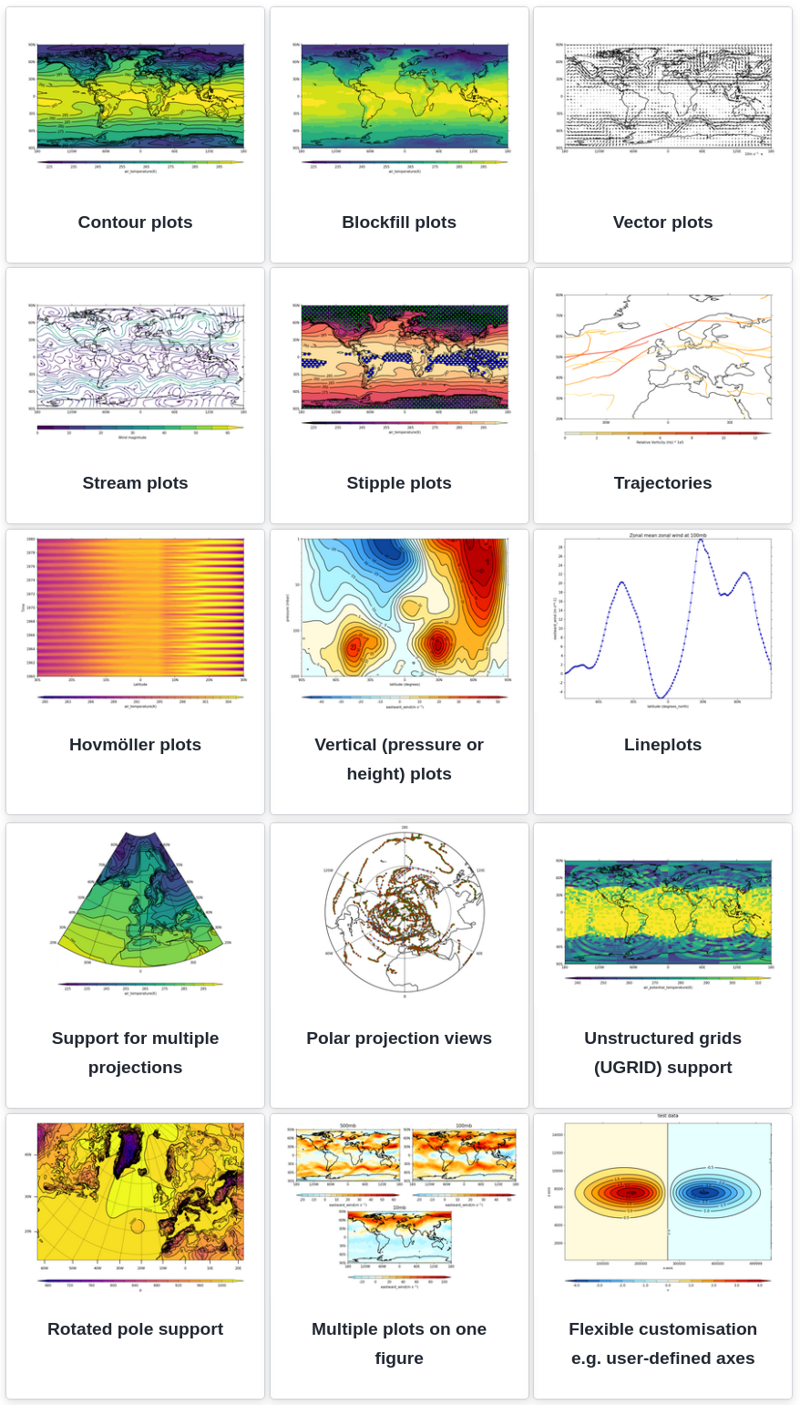
Examples gallery of plots made with the cf-plot library.
See the cf-plot gallery for the wide range of plotting possibilities, with example code. These include, but are not limited to:
Cylindrical, polar stereographic and other plane projections
Latitude or longitude vs. height or pressure
Hovmuller
Vectors
Stipples
Multiple plots on a page
Colour scales
User defined axes
Rotated pole
Irregular grids
Trajectories
Line plots
Field lists
A field list, contained in a cf.FieldList instance, is an ordered
sequence of field constructs. It supports all of the Python list
operations, such as indexing, iteration, and methods like
append.
>>> x = cf.read('file.nc')
>>> y = cf.read('precipitation_flux.nc')
>>> x
[<CF Field: specific_humidity(latitude(5), longitude(8)) 1>,
 <CF Field: air_temperature(atmosphere_hybrid_height_coordinate(1), grid_latitude(10), grid_longitude(9)) K>]
>>> y
[<CF Field: precipitation_flux(time(1), latitude(64), longitude(128)) kg m-2 day-1>]
>>> y.extend(x)
>>> y
[<CF Field: precipitation_flux(time(1), latitude(64), longitude(128)) kg m-2 day-1>,
 <CF Field: specific_humidity(latitude(5), longitude(8)) 1>,
 <CF Field: air_temperature(atmosphere_hybrid_height_coordinate(1), grid_latitude(10), grid_longitude(9)) K>]
>>> y[2]
<CF Field: air_temperature(atmosphere_hybrid_height_coordinate(1), grid_latitude(10), grid_longitude(9)) K>
>>> y[::-1]
[<CF Field: air_temperature(atmosphere_hybrid_height_coordinate(1), grid_latitude(10), grid_longitude(9)) K>,
 <CF Field: specific_humidity(latitude(5), longitude(8)) 1>,
 <CF Field: precipitation_flux(time(1), latitude(64), longitude(128)) kg m-2 day-1>]
>>> len(y)
3
>>> len(y + y)
6
>>> len(y * 4)
12
>>> for f in y:
...     print('field:', repr(f))
...
field: <CF Field: precipitation_flux(time(1), latitude(64), longitude(128)) kg m-2 day-1>
field: <CF Field: specific_humidity(latitude(5), longitude(8)) 1>
field: <CF Field: air_temperature(atmosphere_hybrid_height_coordinate(1), grid_latitude(10), grid_longitude(9)) K>
The field list also has some additional methods for copying, testing equality, sorting and selection.
Properties
Descriptive properties that apply to field construct as a whole may be
retrieved with the properties method:
>>> t = cf.read('file.nc')[1]
>>> t.properties()
{'Conventions': 'CF-1.11',
 'project': 'research',
 'standard_name': 'air_temperature',
 'units': 'K'}
Note
From a Python script or using the standard Python shell, the result of methods such as the property methods given here will be returned in condensed form, without linebreaks between items.
If a “pretty printed” output as displayed in these pages is preferred, use the ipython shell or wrap calls with a suitable method from Python’s dedicated pprint module.
Individual properties may be accessed and modified with the
del_property, get_property, has_property,
and set_property methods:
>>> t.has_property('standard_name')
True
>>> t.get_property('standard_name')
'air_temperature'
>>> t.del_property('standard_name')
'air_temperature'
>>> t.get_property('standard_name', default='not set')
'not set'
>>> t.set_property('standard_name', value='air_temperature')
>>> t.get_property('standard_name', default='not set')
'air_temperature'
A collection of properties may be set at the same time with the
set_properties method of the field construct, and all or some
properties may be removed with the clear_properties and
del_properties methods respectively.
>>> original = t.properties()
>>> original
{'Conventions': 'CF-1.11',
 'project': 'research',
 'standard_name': 'air_temperature',
 'units': 'K'}
>>> t.set_properties({'foo': 'bar', 'units': 'K'})
>>> t.properties()
{'Conventions': 'CF-1.11',
 'foo': 'bar',
 'project': 'research',
 'standard_name': 'air_temperature',
 'units': 'K'}
>>> t.clear_properties()
 {'Conventions': 'CF-1.11',
 'foo': 'bar',
 'project': 'research',
 'standard_name': 'air_temperature',
 'units': 'K'}
>>> t.properties()
{'units': 'K'}
>>> t.set_properties(original)
>>> t.properties()
{'Conventions': 'CF-1.11',
 'project': 'research',
 'standard_name': 'air_temperature',
 'units': 'K'}
Note that the units property persisted after the call to the
clear_properties method because is it deeply associated with
the field construct’s data, which still exists.
All of the methods related to the properties are listed here.
Field identities
A field construct identity is a string that describes the construct
and is based on the field construct’s properties. A canonical identity
is returned by the identity method of the field construct,
and all possible identities are returned by the identities
method.
A field construct’s identity may be any one of the following
The value of the
standard_nameproperty, e.g.'air_temperature',The value of the
idattribute, preceded by'id%=',The value of any property, preceded by the property name and an equals, e.g.
'long_name=Air Temperature','foo=bar', etc.,The netCDF variable name, preceded by “ncvar%”, e.g.
'ncvar%tas'(see the netCDF interface),
>>> t.identity()
'air_temperature'
>>> t.identities()
['air_temperature',
 'Conventions=CF-1.11',
 'project=research',
 'units=K',
 'standard_name=air_temperature',
 'ncvar%ta']
The identity returned by the identity method is, by default,
the least ambiguous identity (defined in the method documentation),
but it may be restricted to the standard_name property and
id attribute; or also the long_name property and
netCDF variable name (see the netCDF interface). See the strict and relaxed keywords.
Metadata constructs
The metadata constructs describe the field construct that contains them. Each CF data model metadata construct has a corresponding cf class:
Class |
CF data model construct |
Description |
|---|---|---|
Domain axis |
Independent axes of the domain |
|
Dimension coordinate |
Domain cell locations |
|
Auxiliary coordinate |
Domain cell locations |
|
Coordinate reference |
Domain coordinate systems |
|
Domain ancillary |
Cell locations in alternative coordinate systems |
|
Cell measure |
Domain cell size or shape |
|
Field ancillary |
Ancillary metadata which vary within the domain |
|
Cell method |
Describes how data represent variation within cells |
Metadata constructs of a particular type can be retrieved with the following attributes of the field construct:
Attribute |
Metadata constructs |
|---|---|
Domain axes |
|
Dimension coordinates |
|
Auxiliary coordinates |
|
Coordinate references |
|
Domain ancillaries |
|
Cell measures |
|
Field ancillaries |
|
Cell methods |
Each of these attributes returns a cf.Constructs class instance that
maps metadata constructs to unique identifiers called “construct
keys”. A cf.Constructs instance has methods for selecting constructs
that meet particular criteria (see
Filtering metadata constructs). It also behaves like a
“read-only” Python dictionary, in that it has items,
keys and values methods that work exactly
like their corresponding dict methods. It also has a
get method and indexing like a Python dictionary (see
Metadata construct access for details).
>>> q, t = cf.read('file.nc')
>>> t.coordinate_references
<CF Constructs: coordinate_reference(2)>
>>> print(t.coordinate_references)
Constructs:
{'coordinatereference0': <CF CoordinateReference: standard_name:atmosphere_hybrid_height_coordinate>,
 'coordinatereference1': <CF CoordinateReference: grid_mapping_name:rotated_latitude_longitude>}
>>> list(t.coordinate_references().keys())
['coordinatereference0', 'coordinatereference1']
>>> for key, value in t.coordinate_references().items():
...     print(key, repr(value))
...
coordinatereference0 <CF CoordinateReference: standard_name:atmosphere_hybrid_height_coordinate>
coordinatereference1 <CF CoordinateReference: grid_mapping_name:rotated_latitude_longitude>
>>> print(t.dimension_coordinates)
Constructs:
{'dimensioncoordinate0': <CF DimensionCoordinate: atmosphere_hybrid_height_coordinate(1) >,
 'dimensioncoordinate1': <CF DimensionCoordinate: grid_latitude(10) degrees>,
 'dimensioncoordinate2': <CF DimensionCoordinate: grid_longitude(9) degrees>,
 'dimensioncoordinate3': <CF DimensionCoordinate: time(1) days since 2018-12-01 >}
>>> print(t.domain_axes)
Constructs:
{'domainaxis0': <CF DomainAxis: size(1)>,
 'domainaxis1': <CF DomainAxis: size(10)>,
 'domainaxis2': <CF DomainAxis: size(9)>,
 'domainaxis3': <CF DomainAxis: size(1)>}
The construct keys (e.g. 'domainaxis1') are usually generated
internally and are unique within the field construct. However,
construct keys may be different for equivalent metadata constructs
from different field constructs, and for different Python sessions.
Metadata constructs of all types may be returned by the
constructs attribute of the field construct:
>>> q.constructs
<CF Constructs: cell_method(1), dimension_coordinate(3), domain_axis(3)>
>>> print(q.constructs)
Constructs:
{'cellmethod0': <CF CellMethod: area: mean>,
 'dimensioncoordinate0': <CF DimensionCoordinate: latitude(5) degrees_north>,
 'dimensioncoordinate1': <CF DimensionCoordinate: longitude(8) degrees_east>,
 'dimensioncoordinate2': <CF DimensionCoordinate: time(1) days since 2018-12-01 >,
 'domainaxis0': <CF DomainAxis: size(5)>,
 'domainaxis1': <CF DomainAxis: size(8)>,
 'domainaxis2': <CF DomainAxis: size(1)>}
>>> t.constructs
<CF Constructs: auxiliary_coordinate(3), cell_measure(1), cell_method(2), coordinate_reference(2), dimension_coordinate(4), domain_ancillary(3), domain_axis(4), field_ancillary(1)>
>>> print(t.constructs)
Constructs:
{'auxiliarycoordinate0': <CF AuxiliaryCoordinate: latitude(10, 9) degrees_N>,
 'auxiliarycoordinate1': <CF AuxiliaryCoordinate: longitude(9, 10) degrees_E>,
 'auxiliarycoordinate2': <CF AuxiliaryCoordinate: long_name=Grid latitude name(10) >,
 'cellmeasure0': <CF CellMeasure: measure:area(9, 10) km2>,
 'cellmethod0': <CF CellMethod: domainaxis1: domainaxis2: mean where land (interval: 0.1 degrees)>,
 'cellmethod1': <CF CellMethod: domainaxis3: maximum>,
 'coordinatereference0': <CF CoordinateReference: standard_name:atmosphere_hybrid_height_coordinate>,
 'coordinatereference1': <CF CoordinateReference: grid_mapping_name:rotated_latitude_longitude>,
 'dimensioncoordinate0': <CF DimensionCoordinate: atmosphere_hybrid_height_coordinate(1) >,
 'dimensioncoordinate1': <CF DimensionCoordinate: grid_latitude(10) degrees>,
 'dimensioncoordinate2': <CF DimensionCoordinate: grid_longitude(9) degrees>,
 'dimensioncoordinate3': <CF DimensionCoordinate: time(1) days since 2018-12-01 >,
 'domainancillary0': <CF DomainAncillary: ncvar%a(1) m>,
 'domainancillary1': <CF DomainAncillary: ncvar%b(1) >,
 'domainancillary2': <CF DomainAncillary: surface_altitude(10, 9) m>,
 'domainaxis0': <CF DomainAxis: size(1)>,
 'domainaxis1': <CF DomainAxis: size(10)>,
 'domainaxis2': <CF DomainAxis: size(9)>,
 'domainaxis3': <CF DomainAxis: size(1)>,
 'fieldancillary0': <CF FieldAncillary: air_temperature standard_error(10, 9) K>}
Data
The field construct’s data is stored in a cf.Data class instance that
is accessed with the data attribute of the field construct.
>>> q, t = cf.read('file.nc')
>>> t.data
<CF Data(1, 10, 9): [[[262.8, ..., 269.7]]] K>
The cf.Data instance provides access to the full array of values, as
well as attributes to describe the array and methods for describing
any data compression. The field construct also
has a get_data method as an alternative means of retrieving
the data instance, which allows for a default to be returned if no
data have been set; as well as a del_data method for removing
the data.
The field construct (and any other construct that contains data) also provides attributes for direct access.
>>> a = t.array
>>> type(a)
numpy.ma.core.MaskedArray
>>> print(a)
[[[262.8 270.5 279.8 269.5 260.9 265.0 263.5 278.9 269.2]
  [272.7 268.4 279.5 278.9 263.8 263.3 274.2 265.7 279.5]
  [269.7 279.1 273.4 274.2 279.6 270.2 280.  272.5 263.7]
  [261.7 260.6 270.8 260.3 265.6 279.4 276.9 267.6 260.6]
  [264.2 275.9 262.5 264.9 264.7 270.2 270.4 268.6 275.3]
  [263.9 263.8 272.1 263.7 272.2 264.2 260.  263.5 270.2]
  [273.8 273.1 268.5 272.3 264.3 278.7 270.6 273.0 270.6]
  [267.9 273.5 279.8 260.3 261.2 275.3 271.2 260.8 268.9]
  [270.9 278.7 273.2 261.7 271.6 265.8 273.  278.5 266.4]
  [276.4 264.2 276.3 266.1 276.1 268.1 277.  273.4 269.7]]]
>>> t.dtype
dtype('float64')
>>> t.ndim
3
>>> t.shape
(1, 10, 9)
>>> t.size
90
The array is stored internally as a Dask array,
which can be retrieved with the to_dask_array() method of the
field construct:
>>> d = t.to_dask_array()
>>> d
dask.array<array, shape=(1, 10, 9), dtype=float64, chunksize=(1, 10, 9), chunktype=numpy.ndarray>
Note that changes to the returned Dask array in-place will also be seen in the field construct.
All of the methods and attributes related to the data are listed here.
Data axes
The data array of the field construct spans all the domain axis
constructs with the possible exception of size one domain axis
constructs. The domain axis constructs spanned by the field
construct’s data are found with the get_data_axes method of
the field construct. For example, the data of the field construct
t does not span the size one domain axis construct with key
'domainaxis3'.
>>> print(t.domain_axes)
Constructs:
{'domainaxis0': <CF DomainAxis: size(1)>,
 'domainaxis1': <CF DomainAxis: size(10)>,
 'domainaxis2': <CF DomainAxis: size(9)>,
 'domainaxis3': <CF DomainAxis: size(1)>}
>>> t
<CF Field: air_temperature(atmosphere_hybrid_height_coordinate(1), grid_latitude(10), grid_longitude(9)) K>
>>> t.data.shape
(1, 10, 9)
>>> t.get_data_axes()
('domainaxis0', 'domainaxis1', 'domainaxis2')
The data may be set with the set_data method of the field
construct. The domain axis constructs spanned by the data are inferred
from the existing domain axis constructs, provided that there are no
ambiguities (such as two dimensions of the same size), in which case
they can be explicitly provided via their construct keys. In any case,
the data axes may be set at any time with the set_data_axes
method of the field construct.
>>> data = t.del_data()
>>> t.has_data()
False
>>> t.set_data(data)
>>> t.data
<CF Data(1, 10, 9): [[[262.8, ..., 269.7]]] K>
See the section field construct creation for more examples.
Date-time
Data representing date-times is defined as elapsed times since a
reference date-time in a particular calendar (Gregorian, by
default). The array attribute of the cf.Data instance
(and any construct that contains it) returns the elapsed times, and
the datetime_array (and any construct that contains it)
returns the data as an array of date-time objects.
>>> d = cf.Data([1, 2, 3], units='days since 2004-2-28')
>>> print(d.array)
[1 2 3]
>>> print(d.datetime_array)
[cftime.DatetimeGregorian(2004-02-29 00:00:00)
 cftime.DatetimeGregorian(2004-03-01 00:00:00)
 cftime.DatetimeGregorian(2004-03-02 00:00:00)]
>>> e = cf.Data([1, 2, 3], units='days since 2004-2-28', calendar='360_day')
>>> print(e.array)
[1 2 3]
>>> print(e.datetime_array)
[cftime.Datetime360Day(2004-02-29 00:00:00)
 cftime.Datetime360Day(2004-02-30 00:00:00)
 cftime.Datetime360Day(2004-03-01 00:00:00)]
Alternatively, date-time data may be created by providing date-time
objects or ISO 8601-like date-time strings. Date-time objects may be
cftime.datetime instances (as returned by the cf.dt and
cf.dt_vector functions), Python datetime.datetime instances, or
any other date-time object that has an equivalent API.
>>> date_time = cf.dt(2004, 2, 29)
>>> date_time
cftime.datetime(2004-02-29 00:00:00)
>>> d = cf.Data(date_time, calendar='gregorian')
>>> print(d.array)
0.0
>>> d.datetime_array
array(cftime.DatetimeGregorian(2004-02-29 00:00:00), dtype=object)
>>> date_times  = cf.dt_vector(['2004-02-29', '2004-02-30', '2004-03-01'], calendar='360_day')
>>> print (date_times)
[cftime.Datetime360Day(2004-02-29 00:00:00)
 cftime.Datetime360Day(2004-02-30 00:00:00)
 cftime.Datetime360Day(2004-03-01 00:00:00)]
>>> e = cf.Data(date_times)
>>> print(e.array)
[0. 1. 2.]
>>> print(e.datetime_array)
[cftime.Datetime360Day(2004-02-29 00:00:00)
 cftime.Datetime360Day(2004-02-30 00:00:00)
 cftime.Datetime360Day(2004-03-01 00:00:00)]
>>> d = cf.Data(['2004-02-29', '2004-02-30', '2004-03-01'], calendar='360_day')
>>> d.Units
<Units: days since 2004-02-29 360_day>
>>> print(d.array)
[0. 1. 2.]
>>> print(d.datetime_array)
[cftime.Datetime360Day(2004-02-29 00:00:00)
 cftime.Datetime360Day(2004-02-30 00:00:00)
 cftime.Datetime360Day(2004-03-01 00:00:00)]
>>> e = cf.Data(['2004-02-29', '2004-03-01', '2004-03-02'], dt=True)
>>> e.Units
<Units: days since 2004-02-29>
>>> print(e.datetime_array)
[cftime.DatetimeGregorian(2004-02-29 00:00:00)
 cftime.DatetimeGregorian(2004-03-01 00:00:00)
 cftime.DatetimeGregorian(2004-03-02 00:00:00)]
>>> f = cf.Data(['2004-02-29', '2004-03-01', '2004-03-02'])
>>> print(f.array)
['2004-02-29' '2004-03-01' '2004-03-02']
>>> f.Units
<Units: >
>>> print(f.datetime_array)  # Raises Exception
Traceback (most recent call last):
    ...
ValueError: Can't create date-time array from units <Units: >
Manipulating dimensions
The dimensions of a field construct’s data may be reordered, have size one dimensions removed and have new size one dimensions included by using the following field construct methods:
Method |
Description |
|---|---|
Flatten domain axes of the field construct |
|
Reverse the direction of a data dimension |
|
Insert a new size one data dimension. The new dimension must correspond to an existing size one domain axis construct. |
|
Remove size one data dimensions |
|
Reorder data dimensions |
|
Insert all missing size one data dimensions |
>>> q, t = cf.read('file.nc')
>>> t
<CF Field: air_temperature(atmosphere_hybrid_height_coordinate(1), grid_latitude(10), grid_longitude(9)) K>
>>> t2 = t.squeeze()
>>> t2
<CF Field: air_temperature(grid_latitude(10), grid_longitude(9)) K>
>>> print(t2.dimension_coordinates)
Constructs:
{'dimensioncoordinate0': <CF DimensionCoordinate: atmosphere_hybrid_height_coordinate(1) >,
 'dimensioncoordinate1': <CF DimensionCoordinate: grid_latitude(10) degrees>,
 'dimensioncoordinate2': <CF DimensionCoordinate: grid_longitude(9) degrees>,
 'dimensioncoordinate3': <CF DimensionCoordinate: time(1) days since 2018-12-01 >}
>>> t3 = t2.insert_dimension(axis='domainaxis3', position=1)
>>> t3
<CF Field: air_temperature(grid_latitude(10), time(1), grid_longitude(9)) K>
>>> t3.transpose([2, 0, 1])
<CF Field: air_temperature(grid_longitude(9), grid_latitude(10), time(1)) K>
When transposing the data dimensions, the dimensions of metadata construct data are, by default, unchanged. It is also possible to permute the data dimensions of the metadata constructs so that they have the same relative order as the field construct:
>>> t4 = t.transpose(['X', 'Z', 'Y'], constructs=True)
Data mask
See also
There is always a data mask, which may be thought of as a separate
data array of Booleans with the same shape as the original data. The
data mask is False where the data has values, and True where
the data is missing. The data mask may be inspected with the
mask attribute of the field construct, which returns the data
mask in a field construct with the same metadata constructs as the
original field construct.
>>> print(q)
Field: specific_humidity (ncvar%q)
----------------------------------
Data            : specific_humidity(latitude(5), longitude(8)) 1
Cell methods    : area: mean
Dimension coords: latitude(5) = [-75.0, ..., 75.0] degrees_north
                : longitude(8) = [22.5, ..., 337.5] degrees_east
                : time(1) = [2019-01-01 00:00:00]
>>> print(q.mask)
Field: long_name=mask
---------------------
Data            : long_name=mask(latitude(5), longitude(8))
Cell methods    : area: mean
Dimension coords: latitude(5) = [-75.0, ..., 75.0] degrees_north
                : longitude(8) = [22.5, ..., 337.5] degrees_east
                : time(1) = [2019-01-01 00:00:00]
>>> print(q.mask.array)
[[False False False False False False False False]
 [False False False False False False False False]
 [False False False False False False False False]
 [False False False False False False False False]
 [False False False False False False False False]]
>>> q[[0, 4], :] = cf.masked
>>> print(q.mask.array)
[[ True  True  True  True  True  True  True  True]
 [False False False False False False False False]
 [False False False False False False False False]
 [False False False False False False False False]
 [ True  True  True  True  True  True  True  True]]
The _FillValue and missing_value attributes of the
field construct are not stored as values of the field construct’s
data. They are only used when writing the data to a netCDF
dataset. Therefore testing for missing
data by testing for equality to one of these property values will
produce incorrect results; the any and all methods
of the field construct should be used instead.
>>> q.mask.all()
False
>>> q.mask.any()
True
The mask of a netCDF dataset array is implied by array values that
meet the criteria implied by the missing_value, _FillValue,
valid_min, valid_max, and valid_range properties, and is
usually applied automatically by cf.read. NetCDF data elements that
equal the values of the missing_value and _FillValue
properties are masked, as are data elements that exceed the value of
the valid_max property, succeed the value of the valid_min
property, or lie outside of the range defined by the valid_range
property.
However, this automatic masking may be bypassed by setting the mask
keyword of the cf.read function to False. The mask, as defined in
the dataset, may subsequently be applied manually with the
apply_masking method of the field construct.
>>> cf.write(q, 'masked_q.nc')
>>> no_mask_q = cf.read('masked_q.nc', mask=False)[0]
>>> print(no_mask_q.array)
[9.96920997e+36, 9.96920997e+36, 9.96920997e+36, 9.96920997e+36,
 9.96920997e+36, 9.96920997e+36, 9.96920997e+36, 9.96920997e+36],
 [0.023 0.036 0.045 0.062 0.046 0.073 0.006 0.066]
 [0.11  0.131 0.124 0.146 0.087 0.103 0.057 0.011]
 [0.029 0.059 0.039 0.07  0.058 0.072 0.009 0.017]
[9.96920997e+36, 9.96920997e+36, 9.96920997e+36, 9.96920997e+36,
 9.96920997e+36, 9.96920997e+36, 9.96920997e+36, 9.96920997e+36]])
>>> masked_q = no_mask_q.apply_masking()
>>> print(masked_q.array)
[[   --    --    --    --    --    --    --    --]
 [0.023 0.036 0.045 0.062 0.046 0.073 0.006 0.066]
 [0.11  0.131 0.124 0.146 0.087 0.103 0.057 0.011]
 [0.029 0.059 0.039 0.07  0.058 0.072 0.009 0.017]
 [   --    --    --    --    --    --    --    --]]
The apply_masking method of the field construct utilises as
many of the missing_value, _FillValue, valid_min,
valid_max, and valid_range properties as are present and may
be used on any construct, not only those that have been read from
datasets.
Subspacing by index
Creation of a new field construct which spans a subspace of the domain of an existing field construct is achieved either by indexing the field construct directly (as described in this section) or by identifying indices based on the metadata constructs (see Subspacing by metadata). The subspacing operation, in either case, also subspaces any metadata constructs of the field construct (e.g. coordinate metadata constructs) which span any of the domain axis constructs that are affected. The new field construct is created with the same properties as the original field construct.
Subspacing by indexing uses rules that are very similar to the numpy indexing rules, the only differences being:
An integer index i specified for a dimension reduces the size of this dimension to unity, taking only the i-th element, but keeps the dimension itself, so that the rank of the array is not reduced.
When two or more dimensions’ indices are sequences of integers then these indices work independently along each dimension (similar to the way vector subscripts work in FORTRAN). This is the same indexing behaviour as on a
Variableobject of the netCDF4 package.
For a dimension that is cyclic, a range of indices specified by a
slicethat spans the edges of the data (such as-2:3or3:-2:-1) is assumed to “wrap” around, rather then producing a null result.
>>> q, t = cf.read('file.nc')
>>> print(q)
Field: specific_humidity (ncvar%q)
----------------------------------
Data            : specific_humidity(latitude(5), longitude(8)) 1
Cell methods    : area: mean
Dimension coords: time(1) = [2019-01-01 00:00:00]
                : latitude(5) = [-75.0, ..., 75.0] degrees_north
                : longitude(8) = [22.5, ..., 337.5] degrees_east

>>> new = q[::-1, 0]
>>> print(new)
Field: specific_humidity (ncvar%q)
----------------------------------
Data            : specific_humidity(latitude(5), longitude(1)) 1
Cell methods    : area: mean
Dimension coords: time(1) = [2019-01-01 00:00:00]
                : latitude(5) = [75.0, ..., -75.0] degrees_north
                : longitude(1) = [22.5] degrees_east
>>> t
<CF Field: air_temperature(atmosphere_hybrid_height_coordinate(1), grid_latitude(10), grid_longitude(9)) K>
>>> t[:, :, 1]
<CF Field: air_temperature(atmosphere_hybrid_height_coordinate(1), grid_latitude(10), grid_longitude(1)) K>
>>> t[:, 0]
<CF Field: air_temperature(atmosphere_hybrid_height_coordinate(1), grid_latitude(1), grid_longitude(9)) K>
>>> t[..., 6:3:-1, 3:6]
<CF Field: air_temperature(atmosphere_hybrid_height_coordinate(1), grid_latitude(3), grid_longitude(3)) K>
>>> t[0, [2, 3, 9], [4, 8]]
<CF Field: air_temperature(atmosphere_hybrid_height_coordinate(1), grid_latitude(3), grid_longitude(2)) K>
>>> t[0, :, -2]
<CF Field: air_temperature(atmosphere_hybrid_height_coordinate(1), grid_latitude(10), grid_longitude(1)) K>
>>> t[..., [True, False, True, True, False, False, True, False, False]]
<CF Field: air_temperature(atmosphere_hybrid_height_coordinate(1), grid_latitude(10), grid_longitude(4)) K>
>>> q
<CF Field: specific_humidity(latitude(5), longitude(8)) 1>
>>> q.cyclic()
{'domainaxis1'}
>>> q.constructs.domain_axis_identity('domainaxis1')
'longitude'
>>> print(q[:, -2:3])
Field: specific_humidity (ncvar%q)
----------------------------------
Data            : specific_humidity(latitude(5), longitude(5)) 1
Cell methods    : area: mean
Dimension coords: latitude(5) = [-75.0, ..., 75.0] degrees_north
                : longitude(5) = [-67.5, ..., 112.5] degrees_east
                : time(1) = [2019-01-01 00:00:00]
>>> print(q[:, 3:-2:-1])
Field: specific_humidity (ncvar%q)
----------------------------------
Data            : specific_humidity(latitude(5), longitude(5)) 1
Cell methods    : area: mean
Dimension coords: latitude(5) = [-75.0, ..., 75.0] degrees_north
                : longitude(5) = [157.5, ..., -22.5] degrees_east
                : time(1) = [2019-01-01 00:00:00]
An index that is a list of integers may also be provided as a numpy
array, a dask array, a cf.Data instance, or a metadata construct
that has data:
>>> lon = q.dimension_coordinate('X')
>>> print(q[:, lon > 180])
Field: specific_humidity (ncvar%q)
----------------------------------
Data            : specific_humidity(latitude(5), longitude(4)) 1
Cell methods    : area: mean
Dimension coords: latitude(5) = [-75.0, ..., 75.0] degrees_north
                : longitude(4) = [202.5, ..., 337.5] degrees_east
                : time(1) = [2019-01-01 00:00:00]
A cf.Data instance can also directly be indexed in the same ways:
>>> t.data[0, [2, 3, 9], [4, 8]]
<CF Data(1, 3, 2): [[[279.6, ..., 269.7]]] K>
Assignment by index
Data elements can be changed by assigning to elements selected by indices of the data (as described in this section); by conditions based on the data values of the field construct or one of its metadata constructs (see Assignment by condition); or by identifying indices based on arbitrary metadata constructs (see Assignment by metadata).
Assignment by indices uses rules that are very similar to the numpy indexing rules, the only difference being:
When two or more dimensions’ indices are sequences of integers then these indices work independently along each dimension (similar to the way vector subscripts work in FORTRAN). This is the same indexing behaviour as on a
Variableobject of the netCDF4 package.
For a dimension that is cyclic, a range of indices specified by a
slicethat spans the edges of the data (such as-2:3or3:-2:-1) is assumed to “wrap” around, rather then producing a null result.
A single value may be assigned to any number of elements.
>>> q, t = cf.read('file.nc')
>>> t[:, 0, 0] = -1
>>> t[:, :, 1] = -2
>>> t[..., 6:3:-1, 3:6] = -3
>>> print(t.array)
[[[ -1.0  -2.0 279.8 269.5 260.9 265.0 263.5 278.9 269.2]
  [272.7  -2.0 279.5 278.9 263.8 263.3 274.2 265.7 279.5]
  [269.7  -2.0 273.4 274.2 279.6 270.2 280.0 272.5 263.7]
  [261.7  -2.0 270.8 260.3 265.6 279.4 276.9 267.6 260.6]
  [264.2  -2.0 262.5  -3.0  -3.0  -3.0 270.4 268.6 275.3]
  [263.9  -2.0 272.1  -3.0  -3.0  -3.0 260.0 263.5 270.2]
  [273.8  -2.0 268.5  -3.0  -3.0  -3.0 270.6 273.0 270.6]
  [267.9  -2.0 279.8 260.3 261.2 275.3 271.2 260.8 268.9]
  [270.9  -2.0 273.2 261.7 271.6 265.8 273.0 278.5 266.4]
  [276.4  -2.0 276.3 266.1 276.1 268.1 277.0 273.4 269.7]]]
An array of values can be assigned, as long as it is broadcastable to the shape defined by the indices, using the numpy broadcasting rules.
>>> import numpy
>>> t[..., 6:3:-1, 3:6] = numpy.arange(9).reshape(3, 3)
>>> t[0, [2, 9], [4, 8]] =  cf.Data([[-4, -5]])
>>> t[0, [4, 7], 0] = [[-10], [-11]]
>>> print(t.array)
[[[ -1.0  -2.0 279.8 269.5 260.9 265.0 263.5 278.9 269.2]
  [272.7  -2.0 279.5 278.9 263.8 263.3 274.2 265.7 279.5]
  [269.7  -2.0 273.4 274.2  -4.0 270.2 280.0 272.5  -5.0]
  [261.7  -2.0 270.8 260.3 265.6 279.4 276.9 267.6 260.6]
  [-10.0  -2.0 262.5   6.0   7.0   8.0 270.4 268.6 275.3]
  [263.9  -2.0 272.1   3.0   4.0   5.0 260.0 263.5 270.2]
  [273.8  -2.0 268.5   0.0   1.0   2.0 270.6 273.0 270.6]
  [-11.0  -2.0 279.8 260.3 261.2 275.3 271.2 260.8 268.9]
  [270.9  -2.0 273.2 261.7 271.6 265.8 273.0 278.5 266.4]
  [276.4  -2.0 276.3 266.1  -4.0 268.1 277.0 273.4  -5.0]]]
In-place modification is also possible:
>>> print(t[0, 0, -1].array)
[[[269.2]]]
>>> t[0, 0, -1] /= -10
>>> print(t[0, 0, -1].array)
[[[-26.92]]]
A cf.Data instance can also assigned values in the same way:
>>> t.data[0, 0, -1] = -99
>>> print(t[0, 0, -1].array)
[[[-99.]]]
An index that is a list of integers may also be provided as a numpy
array, a dask array, a cf.Data instance, or a metadata construct
that has data:
>>> y = t.dimension_coordinate('Y')
>>> t[:, y > 0] = -6
>>> print(t)
[[[ -6.0 -4.0  -6.0  -6.0  -6.0  -6.0  -6.0  -6.0  -6.0]
  [ -6.0 -4.0  -6.0  -6.0  -6.0  -6.0  -6.0  -6.0  -6.0]
  [ -6.0 -4.0  -6.0  -6.0  -6.0  -6.0  -6.0  -6.0  -6.0]
  [ -6.0 -4.0  -6.0  -6.0  -6.0  -6.0  -6.0  -6.0  -6.0]
  [ -6.0 -4.0  -6.0  -6.0  -6.0  -6.0  -6.0  -6.0  -6.0]
  [263.9 -2.0 272.1   3.0   4.0   5.0 260.0 263.5 270.2]
  [273.8 -2.0 268.5   0.0   1.0   2.0 270.6 273.0 270.6]
  [-11.0 -2.0 279.8 260.3 261.2 275.3 271.2 260.8 268.9]
  [270.9 -2.0 273.2 261.7 271.6 265.8 273.0 278.5 266.4]
  [276.4 -2.0 276.3 266.1  -4.0 268.1 277.0 273.4  -5.0]]]
Masked values
Data array elements may be set to masked values by assigning them to
the cf.masked constant, thereby updating the data mask.
>>> t[0, :, -2] = cf.masked
>>> print(t.array)
[[[ -1.0  -2.0 279.8 269.5 260.9 265.0 263.5    -- -99.0]
  [272.7  -2.0 279.5 278.9 263.8 263.3 274.2    -- 279.5]
  [269.7  -2.0 273.4 274.2  -4.0 270.2 280.0    --  -5.0]
  [261.7  -2.0 270.8 260.3 265.6 279.4 276.9    -- 260.6]
  [264.2  -2.0 262.5   6.0   7.0   8.0 270.4    -- 275.3]
  [263.9  -2.0 272.1   3.0   4.0   5.0 260.0    -- 270.2]
  [273.8  -2.0 268.5   0.0   1.0   2.0 270.6    -- 270.6]
  [-11.0  -2.0 279.8 260.3 261.2 275.3 271.2    -- 268.9]
  [270.9  -2.0 273.2 261.7 271.6 265.8 273.0    -- 266.4]
  [276.4  -2.0 276.3 266.1  -4.0 268.1 277.0    --  -5.0]]]
By default the data mask is “hard”, meaning that masked values can not
be changed by assigning them to another value. This behaviour may be
changed by setting the hardmask attribute of the field
construct to False, thereby making the data mask “soft”.
>>> t[0, 4, -2] = 99
>>> print(t[0, 4, -2].array)
[[[--]]]
>>> t.hardmask = False
>>> t[0, 4, -2] = 99
>>> print(t[0, 4, -2].array)
[[[99.]]]
Note that this is the opposite behaviour to numpy arrays, which
assume that the mask is soft by default. The
reason for the difference is so that land-sea masks are, by default,
preserved through assignment operations.
Assignment from other field constructs
Another field construct can also be assigned to indices. The other field construct’s data is actually assigned, but only after being transformed so that it is broadcastable to the subspace defined by the assignment indices. This is done by using the metadata constructs of the two field constructs to create a mapping of physically compatible dimensions between the fields, and then manipulating the dimensions of the other field construct’s data to ensure that they are broadcastable.
>>> q, t = cf.read('file.nc')
>>> t0 = t.copy()
>>> u = t.squeeze(0)
>>> u.transpose(inplace=True)
>>> u.flip(inplace=True)
>>> t[...] = u
>>> t.allclose(t0)
True
>>> print(t[:, :, 1:3].array)
[[[270.5 279.8]
   [268.4 279.5]
   [279.1 273.4]
   [260.6 270.8]
   [275.9 262.5]
   [263.8 272.1]
   [273.1 268.5]
   [273.5 279.8]
   [278.7 273.2]
   [264.2 276.3]]]
>>> print(u[2].array)
[[277.  273.  271.2 270.6 260.  270.4 276.9 280.  274.2 263.5]]
>>> t[:, :, 1:3] = u[2]
>>> print(t[:, :, 1:3].array)
[[[263.5 263.5]
  [274.2 274.2]
  [280.  280. ]
  [276.9 276.9]
  [270.4 270.4]
  [260.  260. ]
  [270.6 270.6]
  [271.2 271.2]
  [273.  273. ]
  [277.  277. ]]]
If either of the field constructs does not have sufficient metadata to
create the such a mapping, then any manipulation of the dimensions
must be done manually, and the other field construct’s cf.Data instance
(rather than the field construct itself) may be assigned.
Assignment of bounds
When assigning an object that has bounds to an object that also has bounds, then the bounds are also assigned. This is the only circumstance that allows bounds to be updated during assignment by index.
Units
The field construct, and any metadata construct that contains data,
has units which are described by the Units attribute that
stores a cf.Units object (which is identical to a cfunits.Units
object of the cfunits package). The units property
provides the units contained in the cf.Units instance, and changes
in one are reflected in the other.
>>> q, t = cf.read('file.nc')
>>> t.units
'K'
>>> t.Units
<Units: K>
>>> t.units = 'degreesC'
>>> t.units
'degreesC'
>>> t.Units
<Units: degreesC>
>>> t.Units += 273.15
>>> t.units
'K'
>>> t.Units
<Units: K>
When the units are changed, the data are automatically converted to the new units when next accessed.
>>> t.data
<CF Data(1, 10, 9): [[[262.8, ..., 269.7]]] K>
>>> t.Units = cf.Units('degreesC')
>>> t.data
<CF Data(1, 10, 9): [[[-10.35, ..., -3.45]]] degreesC>
>>> t.units = 'Kelvin'
>>> t.data
<CF Data(1, 10, 9): [[[262.8, ..., 269.7]]] Kelvin>
When assigning to the data with values that have units, the values are automatically converted to have the same units as the data.
>>> t.data
<CF Data(1, 10, 9): [[[262.8, ..., 269.7]]] Kelvin>
>>> t[0, 0, 0] = cf.Data(1)
>>> t.data
<CF Data(1, 10, 9): [[[1.0, ..., 269.7]]] Kelvin>
>>> t[0, 0, 0] = cf.Data(1, 'degreesC')
>>> t.data
<CF Data(1, 10, 9): [[[274.15, ..., 269.7]]] Kelvin>
Automatic units conversions are also carried out between operands during mathematical operations.
Calendar
When the data represents date-times, the cf.Units instance describes
both the units and calendar of the data. If the latter is missing then
the Gregorian calendar is assumed, as per the CF conventions. The
calendar property provides the calendar contained in the
cf.Units instance, and changes in one are reflected in the other.
>>> air_temp = cf.read('air_temperature.nc')[0]
>>> time = air_temp.coordinate('time')
>>> time.units
'days since 1860-1-1'
>>> time.calendar
'360_day'
>>> time.Units
<Units: days since 1860-1-1 360_day>
Filtering metadata constructs
A cf.Constructs instance has filtering methods for selecting
constructs that meet various criteria:
Method |
Filter criteria |
|---|---|
|
General purpose interface to all other filter methods |
Metadata construct identity |
|
Metadata construct type |
|
Property values |
|
The domain axis constructs spanned by the data |
|
The number of domain axis constructs spanned by the data |
|
The size domain axis constructs |
|
Measure value (for cell measure constructs) |
|
Method value (for cell method constructs) |
|
Whether or not there could be be data. |
|
Construct key |
|
NetCDF variable name (see the netCDF interface) |
|
NetCDF dimension name (see the netCDF interface) |
The filter method of a Constructs instance allows
these filters to be chained together in a single call.
Each of these methods returns a new cf.Constructs instance that
contains the selected metadata constructs.
>>> q, t = cf.read('file.nc')
>>> print(t.constructs.filter_by_type('dimension_coordinate'))
Constructs:
{'dimensioncoordinate0': <CF DimensionCoordinate: atmosphere_hybrid_height_coordinate(1) >,
 'dimensioncoordinate1': <CF DimensionCoordinate: grid_latitude(10) degrees>,
 'dimensioncoordinate2': <CF DimensionCoordinate: grid_longitude(9) degrees>,
 'dimensioncoordinate3': <CF DimensionCoordinate: time(1) days since 2018-12-01 >}
>>> print(t.constructs.filter_by_type('cell_method', 'field_ancillary'))
Constructs:
{'cellmethod0': <CF CellMethod: domainaxis1: domainaxis2: mean where land (interval: 0.1 degrees)>,
 'cellmethod1': <CF CellMethod: domainaxis3: maximum>,
 'fieldancillary0': <CF FieldAncillary: air_temperature standard_error(10, 9) K>}
>>> print(t.constructs.filter_by_property(
...             standard_name='air_temperature standard_error'))
Constructs:
{'fieldancillary0': <CF FieldAncillary: air_temperature standard_error(10, 9) K>}
>>> print(t.constructs.filter_by_property(
...             standard_name='air_temperature standard_error',
...             units='K'))
Constructs:
{'fieldancillary0': <CF FieldAncillary: air_temperature standard_error(10, 9) K>}
>>> print(t.constructs.filter_by_property(
...             'or',
...             standard_name='air_temperature standard_error',
...             units='m'))
Constructs:
{'domainancillary0': <CF DomainAncillary: ncvar%a(1) m>,
 'domainancillary2': <CF DomainAncillary: surface_altitude(10, 9) m>,
 'fieldancillary0': <CF FieldAncillary: air_temperature standard_error(10, 9) K>}
>>> print(t.constructs.filter_by_axis('X', 'Y', axis_mode='or'))
Constructs:
{'auxiliarycoordinate0': <CF AuxiliaryCoordinate: latitude(10, 9) degrees_N>,
 'auxiliarycoordinate1': <CF AuxiliaryCoordinate: longitude(9, 10) degrees_E>,
 'auxiliarycoordinate2': <CF AuxiliaryCoordinate: long_name=Grid latitude name(10) >,
 'cellmeasure0': <CF CellMeasure: measure:area(9, 10) km2>,
 'dimensioncoordinate1': <CF DimensionCoordinate: grid_latitude(10) degrees>,
 'domainancillary2': <CF DomainAncillary: surface_altitude(10, 9) m>,
 'fieldancillary0': <CF FieldAncillary: air_temperature standard_error(10, 9) K>}
>>> print(t.constructs.filter_by_measure('area'))
Constructs:
{'cellmeasure0': <CF CellMeasure: measure:area(9, 10) km2>}
>>> print(t.constructs.filter_by_method('maximum'))
Constructs:
{'cellmethod1': <CF CellMethod: domainaxis3: maximum>}
As each of these methods returns a cf.Constructs instance, further
filters can be performed directly on their results:
>>> print(
...     t.constructs.filter_by_type('auxiliary_coordinate').filter_by_axis('domainaxis2')
... )
Constructs:
{'auxiliarycoordinate0': <CF AuxiliaryCoordinate: latitude(10, 9) degrees_N>,
 'auxiliarycoordinate1': <CF AuxiliaryCoordinate: longitude(9, 10) degrees_E>}
>>> c = t.constructs.filter_by_type('dimension_coordinate')
>>> d = c.filter_by_property(units='degrees')
>>> print(d)
Constructs:
{'dimensioncoordinate1': <CF DimensionCoordinate: grid_latitude(10) degrees>,
 'dimensioncoordinate2': <CF DimensionCoordinate: grid_longitude(9) degrees>}
Construct identities
Another method of selection is by metadata construct “identity”.
Construct identities are used to describe constructs when they are
inspected, and so it is often convenient to copy these identities when
selecting metadata constructs. For example, the three auxiliary
coordinate constructs in the field construct t
have identities 'latitude', 'longitude' and 'long_name=Grid
latitude name'.
A construct’s identity may be any one of the following
The value of the
standard_nameproperty, e.g.'air_temperature',The value of the
idattribute, preceded by'id%=',The physical nature of the construct denoted by
'X','Y','Z'or'T', denoting longitude (or x-projection), latitude (or y-projection), vertical and temporal constructs respectively,The value of any property, preceded by the property name and an equals, e.g.
'long_name=Air Temperature','axis=X','foo=bar', etc.,The cell measure, preceded by “measure:”, e.g.
'measure:volume'The cell method, preceded by “method:”, e.g.
'method:maximum'The netCDF variable name, preceded by “ncvar%”, e.g.
'ncvar%tas'(see the netCDF interface),The netCDF dimension name, preceded by “ncdim%” e.g.
'ncdim%z'(see the netCDF interface), andThe construct key, optionally preceded by “key%”, e.g.
'auxiliarycoordinate2'or'key%auxiliarycoordinate2'.
>>> print(t)
Field: air_temperature (ncvar%ta)
---------------------------------
Data            : air_temperature(atmosphere_hybrid_height_coordinate(1), grid_latitude(10), grid_longitude(9)) K
Cell methods    : grid_latitude(10): grid_longitude(9): mean where land (interval: 0.1 degrees) time(1): maximum
Field ancils    : air_temperature standard_error(grid_latitude(10), grid_longitude(9)) = [[0.81, ..., 0.78]] K
Dimension coords: time(1) = [2019-01-01 00:00:00]
                : atmosphere_hybrid_height_coordinate(1) = [1.5]
                : grid_latitude(10) = [2.2, ..., -1.76] degrees
                : grid_longitude(9) = [-4.7, ..., -1.18] degrees
Auxiliary coords: latitude(grid_latitude(10), grid_longitude(9)) = [[53.941, ..., 50.225]] degrees_N
                : longitude(grid_longitude(9), grid_latitude(10)) = [[2.004, ..., 8.156]] degrees_E
                : long_name=Grid latitude name(grid_latitude(10)) = [--, ..., 'kappa']
Cell measures   : measure:area(grid_longitude(9), grid_latitude(10)) = [[2391.9657, ..., 2392.6009]] km2
Coord references: grid_mappng_name:rotated_latitude_longitude
                : standard_name:atmosphere_hybrid_height_coordinate
Domain ancils   : ncvar%a(atmosphere_hybrid_height_coordinate(1)) = [10.0] m
                : ncvar%b(atmosphere_hybrid_height_coordinate(1)) = [20.0]
                : surface_altitude(grid_latitude(10), grid_longitude(9)) = [[0.0, ..., 270.0]] m
>>> print(t.constructs.filter_by_identity('X'))
Constructs:
{'auxiliarycoordinate1': <CF AuxiliaryCoordinate: longitude(9, 10) degrees_E>,
 'dimensioncoordinate2': <CF DimensionCoordinate: grid_longitude(9) degrees>}
>>> print(t.constructs.filter_by_identity('latitude'))
Constructs:
{'auxiliarycoordinate0': <CF AuxiliaryCoordinate: latitude(10, 9) degrees_N>}
>>> print(t.constructs.filter_by_identity('long_name=Grid latitude name'))
Constructs:
{'auxiliarycoordinate2': <CF AuxiliaryCoordinate: long_name=Grid latitude name(10) >}
>>> print(t.constructs.filter_by_identity('measure:area'))
Constructs:
{'cellmeasure0': <CF CellMeasure: measure:area(9, 10) km2>}
>>> print(t.constructs.filter_by_identity('ncvar%b'))
Constructs:
{'domainancillary1': <CF DomainAncillary: ncvar%b(1) >}
The identity returned by the identity method is, by default, the
least ambiguous identity (defined in the method documentation), but it
may be restricted in various ways. See the strict and relaxed
keywords.
As a further convenience, selection by construct identity is also
possible by providing identities to a call of a cf.Constructs
instance itself, and this technique for selecting constructs by
identity will be used in the rest of this tutorial:
>>> print(t.constructs.filter_by_identity('latitude'))
Constructs:
{'auxiliarycoordinate0': <CF AuxiliaryCoordinate: latitude(10, 9) degrees_N>}
>>> print(t.constructs('latitude'))
Constructs:
{'auxiliarycoordinate0': <CF AuxiliaryCoordinate: latitude(10, 9) degrees_N>}
Selection by construct key is useful for systematic metadata construct access, or for when a metadata construct is not identifiable by other means:
>>> print(t.constructs.filter_by_key('domainancillary2'))
Constructs:
{'domainancillary2': <CF DomainAncillary: surface_altitude(10, 9) m>}
>>> print(t.constructs.filter_by_key('cellmethod1'))
Constructs:
{'cellmethod1': <CF CellMethod: domainaxis3: maximum>}
>>> print(t.constructs.filter_by_key('auxiliarycoordinate2', 'cellmeasure0'))
Constructs:
{'auxiliarycoordinate2': <CF AuxiliaryCoordinate: long_name=Grid latitude name(10) >,
 'cellmeasure0': <CF CellMeasure: measure:area(9, 10) km2>}
If no constructs match the given criteria, then an “empty”
cf.Constructs instance is returned:
>>> c = t.constructs('radiation_wavelength')
>>> c
<CF Constructs: >
>>> print(c)
Constructs:
{}
>>> len(c)
0
The constructs that were not selected by a filter may be returned by
the inverse_filter method applied to the results of
filters:
>>> c = t.constructs.filter_by_type('auxiliary_coordinate')
>>> c
<CF Constructs: auxiliary_coordinate(3)>
>>> c.inverse_filter()
<CF Constructs: cell_measure(1), cell_method(2), coordinate_reference(2), dimension_coordinate(4), domain_ancillary(3), domain_axis(4), field_ancillary(1)>
Note that selection by construct type is equivalent to using the particular method of the field construct for retrieving that type of metadata construct:
>>> print(t.constructs.filter_by_type('cell_measure'))
Constructs:
{'cellmeasure0': <CF CellMeasure: measure:area(9, 10) km2>}
>>> print(t.cell_measures)
Constructs:
{'cellmeasure0': <CF CellMeasure: measure:area(9, 10) km2>}
Metadata construct access
An individual metadata construct, or its construct key, may be returned by any of the following techniques:
with the
constructmethod of a field construct,
>>> t.construct('latitude')
<CF AuxiliaryCoordinate: latitude(10, 9) degrees_N>
>>> t.construct('latitude', key=True)
'auxiliarycoordinate0'
with the
construct_keymethod of a field construct:
>>> key = t.construct_key('latitude')
>>> t.get_construct(key)
<CF AuxiliaryCoordinate: latitude(10, 9) degrees_N>
with the
construct_itemmethod of a field construct:
>>> key, lat = t.construct_item('latitude')
('auxiliarycoordinate0', <AuxiliaryCoordinate: latitude(10, 9) degrees_N>)
by indexing a
cf.Constructsinstance with a construct key.
>>> t.constructs[key]
<CF AuxiliaryCoordinate: latitude(10, 9) degrees_N>
with the
getmethod of acf.Constructsinstance, or
>>> t.constructs.get(key)
<CF AuxiliaryCoordinate: latitude(10, 9) degrees_N>
In addition, an individual metadata construct of a particular type can be retrieved with the following methods of the field construct:
Method |
Metadata construct |
|---|---|
Domain axis |
|
Dimension coordinate |
|
Auxiliary coordinate |
|
Coordinate reference |
|
Domain ancillary |
|
Cell measure |
|
Field ancillary |
|
Cell method |
These methods will only look for the given identity amongst constructs of the chosen type.
>>> t.auxiliary_coordinate('latitude')
<CF AuxiliaryCoordinate: latitude(10, 9) degrees_N>
>>> t.auxiliary_coordinate('latitude', key=True)
'auxiliarycoordinate0'
>>> t.auxiliary_coordinate('latitude', item=True)
('auxiliarycoordinate0', <CF AuxiliaryCoordinate: latitude(10, 9) degrees_N>)
The construct method of the field construct, the above
methods for finding a construct of a particular type, and the
value method of the cf.Constructs instance will all
raise an exception of there is not a unique metadata construct to
return, but this may be replaced with returning a default value or
raising a customised exception:
>>> t.construct('measure:volume')                # Raises Exception
Traceback (most recent call last):
   ...
ValueError: Can't return zero constructs
>>> t.construct('measure:volume', default=False)
False
>>> t.construct('measure:volume', default=Exception("my error"))  # Raises Exception
Traceback (most recent call last):
   ...
Exception: my error
>>> c = t.constructs.filter_by_measure("volume")
>>> len(c)
0
>>> d = t.constructs("units=degrees")
>>> len(d)
2
>>> t.construct("units=degrees")  # Raises Exception
Traceback (most recent call last):
   ...
ValueError: Field.construct() can't return 2 constructs
>>> print(t.construct("units=degrees", default=None))
None
The get method of a cf.Constructs instance accepts an
optional second argument to be returned if the construct key does not
exist, exactly like the Python dict.get method.
Metadata construct properties
Metadata constructs share the same API as the field construct for accessing their properties:
>>> lon = q.construct('longitude')
>>> lon
<CF DimensionCoordinate: longitude(8) degrees_east>
>>> lon.set_property('long_name', 'Longitude')
>>> lon.properties()
{'units': 'degrees_east',
 'long_name': 'Longitude',
 'standard_name': 'longitude'}
>>> area = t.constructs.filter_by_property(units='km2').value()
>>> area
<CF CellMeasure: measure:area(9, 10) km2>
>>> area.identity()
'measure:area'
>>> area.identities()
['measure:area', 'units=km2', 'ncvar%cell_measure']
Metadata construct data
Metadata constructs share the a similar API as the field construct as the field construct for accessing their data:
>>> lon = q.constructs('longitude').value()
>>> lon
<CF DimensionCoordinate: longitude(8) degrees_east>
>>> lon.data
<CF Data(8): [22.5, ..., 337.5] degrees_east>
>>> lon.data[2]
<CF Data(1): [112.5] degrees_east>
>>> lon.data[2] = 133.33
>>> print(lon.array)
[ 22.5   67.5  133.33 157.5  202.5  247.5  292.5  337.5 ]
>>> lon.data[2] = 112.5
The domain axis constructs spanned by a particular metadata
construct’s data are found with the get_data_axes method
of the field construct:
>>> key = t.construct_key('latitude')
>>> key
'auxiliarycoordinate0'
>>> t.get_data_axes(key)
('domainaxis1', 'domainaxis2')
The domain axis constructs spanned by all the data of all metadata
construct may be found with the data_axes method of the
field construct’s cf.Constructs instance:
>>> t.constructs.data_axes()
{'auxiliarycoordinate0': ('domainaxis1', 'domainaxis2'),
 'auxiliarycoordinate1': ('domainaxis2', 'domainaxis1'),
 'auxiliarycoordinate2': ('domainaxis1',),
 'cellmeasure0': ('domainaxis2', 'domainaxis1'),
 'dimensioncoordinate0': ('domainaxis0',),
 'dimensioncoordinate1': ('domainaxis1',),
 'dimensioncoordinate2': ('domainaxis2',),
 'dimensioncoordinate3': ('domainaxis3',),
 'domainancillary0': ('domainaxis0',),
 'domainancillary1': ('domainaxis0',),
 'domainancillary2': ('domainaxis1', 'domainaxis2'),
 'fieldancillary0': ('domainaxis1', 'domainaxis2')}
A size one domain axis construct that is not spanned by the field
construct’s data may still be spanned by the data of metadata
constructs. For example, the data of the field construct t
does not span the size one domain axis construct
with key 'domainaxis3', but this domain axis construct is spanned
by a “time” dimension coordinate construct (with key
'dimensioncoordinate3'). Such a dimension coordinate (i.e. one
that applies to a domain axis construct that is not spanned by the
field construct’s data) corresponds to a CF-netCDF scalar coordinate
variable.
Time
Constructs (including the field constructs) that represent elapsed
time have data array values that provide elapsed time since a
reference date. These constructs are identified by the presence of
“reference time” units. The data values may be converted into the
date-time objects of the cftime package with the datetime_array
attribute of the construct, or its cf.Data instance.
>>> time = q.construct('time')
>>> time
<CF DimensionCoordinate: time(1) days since 2018-12-01 >
>>> time.get_property('units')
'days since 2018-12-01'
>>> time.get_property('calendar', default='standard')
'standard'
>>> print(time.array)
[31.]
>>> print(time.datetime_array)
[cftime.DatetimeGregorian(2019-01-01 00:00:00)]
Time duration
A period of time may stored in a cf.TimeDuration object. For many
applications, a cf.Data instance with appropriate units (such as
seconds) is equivalent, but a cf.TimeDuration instance also
allows units of calendar years or months; and may be relative to a
date-time offset.
>>> cm = cf.TimeDuration(1, 'calendar_month', day=16, hour=12)
>>> cm
<CF TimeDuration: P1M (Y-M-16 12:00:00)>
cf.TimeDuration objects support comparison and arithmetic operations
with numeric scalars, cf.Data instances and date-time objects:
>>> cf.dt(2000, 2, 1) + cm
cftime.datetime(2000-03-01 00:00:00)
>>> cf.Data([1, 2, 3], 'days since 2000-02-01') + cm
<CF Data(3): [2000-03-02 00:00:00, 2000-03-03 00:00:00, 2000-03-04 00:00:00] gregorian>
Date-time ranges that span the time duration can also be created:
>>> cm.interval(cf.dt(2000, 2, 1))
(cftime.DatetimeGregorian(2000-02-01 00:00:000),
 cftime.DatetimeGregorian(2000-03-01 00:00:000))
>>> cm.bounds(cf.dt(2000, 2, 1))
(cftime.DatetimeGregorian(2000-01-16 12:00:00),
 cftime.DatetimeGregorian(2000-02-16 12:00:00))
Time duration constructors
For convenience, cf.TimeDuration instances can be created with the
following constructors:
Constructor |
Description |
|---|---|
A |
|
A |
|
A |
|
A |
|
A |
|
A |
>>> cf.D()
<CF TimeDuration: P1D (Y-M-D 00:00:00)>
>>> cf.Y(10, month=12)
<CF TimeDuration: P10Y (Y-12-01 00:00:00)>

----
Domain
The domain of the CF data model is defined
collectively by various other metadata constructs. It is represented
by the Domain class. A domain construct may exist independently, or
is accessed from a field construct with its domain attribute,
or get_domain method.
>>> domain = t.domain
>>> domain
<CF Domain: {1, 1, 9, 10}>
>>> print(domain)
Dimension coords: atmosphere_hybrid_height_coordinate(1) = [1.5]
                : grid_latitude(10) = [2.2, ..., -1.76] degrees
                : grid_longitude(9) = [-4.7, ..., -1.18] degrees
                : time(1) = [2019-01-01 00:00:00]
Auxiliary coords: latitude(grid_latitude(10), grid_longitude(9)) = [[53.941, ..., 50.225]] degrees_N
                : longitude(grid_longitude(9), grid_latitude(10)) = [[2.004, ..., 8.156]] degrees_E
                : long_name=Grid latitude name(grid_latitude(10)) = [--, ..., 'kappa']
Cell measures   : measure:area(grid_longitude(9), grid_latitude(10)) = [[2391.9657, ..., 2392.6009]] km2
Coord references: grid_mapping_name:rotated_latitude_longitude
                : standard_name:atmosphere_hybrid_height_coordinate
Domain ancils   : ncvar%a(atmosphere_hybrid_height_coordinate(1)) = [10.0] m
                : ncvar%b(atmosphere_hybrid_height_coordinate(1)) = [20.0]
                : surface_altitude(grid_latitude(10), grid_longitude(9)) = [[0.0, ..., 270.0]] m
>>> description = domain.dump(display=False)
Changes to domain instance are seen by the field construct, and vice versa. This is because the domain instance is merely a “view” of the relevant metadata constructs contained in the field construct.
>>> domain_latitude = t.domain.constructs('latitude').value()
>>> field_latitude = t.constructs('latitude').value()
>>> domain_latitude.set_property('test', 'set by domain')
>>> print(field_latitude.get_property('test'))
set by domain
>>> field_latitude.set_property('test', 'set by field')
>>> print(domain_latitude.get_property('test'))
set by field
>>> domain_latitude.del_property('test')
'set by field'
>>> field_latitude.has_property('test')
False
All of the methods and attributes related to the domain are listed here.
Metadata construct types
Domain axes
A domain axis metadata construct specifies the number of points along
an independent axis of the field construct’s domain and is stored in a
cf.DomainAxis instance. The size of the axis is retrieved with
the get_size method of the domain axis construct.
>>> print(q.domain_axes)
Constructs:
{'domainaxis0': <CF DomainAxis: size(5)>,
 'domainaxis1': <CF DomainAxis: size(8)>,
 'domainaxis2': <CF DomainAxis: size(1)>}
>>> d = q.domain_axes().get('domainaxis1')
>>> d
<CF DomainAxis: size(8)>
>>> d.get_size()
8
Coordinates
There are two types of coordinate construct, dimension and auxiliary
coordinate constructs, which can be retrieved together with the
coordinates method of the field construct, as well as
individually with the auxiliary_coordinates and
dimension_coordinates methods.
>>> print(t.coordinates)
Constructs:
{'auxiliarycoordinate0': <CF AuxiliaryCoordinate: latitude(10, 9) degrees_N>,
 'auxiliarycoordinate1': <CF AuxiliaryCoordinate: longitude(9, 10) degrees_E>,
 'auxiliarycoordinate2': <CF AuxiliaryCoordinate: long_name=Grid latitude name(10) >,
 'dimensioncoordinate0': <CF DimensionCoordinate: atmosphere_hybrid_height_coordinate(1) >,
 'dimensioncoordinate1': <CF DimensionCoordinate: grid_latitude(10) degrees>,
 'dimensioncoordinate2': <CF DimensionCoordinate: grid_longitude(9) degrees>,
 'dimensioncoordinate3': <CF DimensionCoordinate: time(1) days since 2018-12-01 >}
Bounds
A coordinate construct may contain an array of cell bounds that
provides the extent of each cell by defining the locations of the cell
vertices. This is in addition to the main data array that contains a
grid point location for each cell. The cell bounds are stored in a
cf.Bounds class instance that is accessed with the
bounds attribute, or get_bounds method, of
the coordinate construct.
A cf.Bounds instance shares the same API as the field
construct for accessing its data.
>>> lon = t.constructs('grid_longitude').value()
>>> bounds = lon.bounds
>>> bounds
<CF Bounds: grid_longitude(9, 2) degrees>
>>> bounds.data
<CF Data(9, 2): [[-4.92, ..., -0.96]] degrees>
>>> print(bounds.array)
[[-4.92 -4.48]
 [-4.48 -4.04]
 [-4.04 -3.6 ]
 [-3.6  -3.16]
 [-3.16 -2.72]
 [-2.72 -2.28]
 [-2.28 -1.84]
 [-1.84 -1.4 ]
 [-1.4  -0.96]]
The cf.Bounds instance inherits the descriptive properties from its
parent coordinate construct, but it may also have its own properties
(although setting these is not recommended).
>>> bounds.inherited_properties()
{'standard_name': 'grid_longitude',
 'units': 'degrees'}
>>> bounds.properties()
{'units': 'degrees'}
Geometry cells
For many geospatial applications, cell bounds can not be represented by a simple line or polygon, and different cells may have different numbers of nodes describing their bounds. For example, if each cell describes the areal extent of a watershed, then it is likely that some watersheds will require more nodes than others. Such cells are called geometries.
If a coordinate construct represents geometries then it will have a
“geometry” attribute (not a CF property) with one of the values 'point',
‘line' or 'polygon'.
This is illustrated with the file geometry.nc (found in the
sample datasets):
>>> f = cf.read('geometry.nc')[0]
>>> print(f)
Field: preciptitation_amount (ncvar%pr)
---------------------------------------
Data            : preciptitation_amount(cf_role=timeseries_id(2), time(4))
Dimension coords: time(4) = [2000-01-02 00:00:00, ..., 2000-01-05 00:00:00]
Auxiliary coords: latitude(cf_role=timeseries_id(2)) = [25.0, 7.0] degrees_north
                : longitude(cf_role=timeseries_id(2)) = [10.0, 40.0] degrees_east
                : altitude(cf_role=timeseries_id(2)) = [5000.0, 20.0] m
                : cf_role=timeseries_id(cf_role=timeseries_id(2)) = [b'x1', b'y2']
Coord references: grid_mapping_name:latitude_longitude
>>> lon = f.auxiliary_coordinate('X')
>>> lon.dump()
Auxiliary coordinate: longitude
   standard_name = 'longitude'
   units = 'degrees_east'
   Data(2) = [10.0, 40.0] degrees_east
   Geometry: polygon
   Bounds:axis = 'X'
   Bounds:standard_name = 'longitude'
   Bounds:units = 'degrees_east'
   Bounds:Data(2, 3, 4) = [[[20.0, ..., --]]] degrees_east
   Interior Ring:Data(2, 3) = [[0, ..., --]]
>>> lon.get_geometry()
'polygon'
Bounds for geometry cells are also stored in a Bounds instance, but
one that always has two extra trailing dimensions (rather than
one). The fist trailing dimension indexes the distinct parts of a
geometry, and the second indexes the nodes of each part. When a part
has fewer nodes than another, its nodes dimension is padded with
missing data.
>>> print(lon.bounds.data.array)
[[20.0 10.0  0.0   --]
 [ 5.0 10.0 15.0 10.0]
 [20.0 10.0  0.0   --]]

[[50.0 40.0 30.0   --]
 [  --   --   --   --]
 [  --   --   --   --]]]
If a cell is composed of multiple polygon parts, an individual polygon
may define an “interior ring”, i.e. a region that is to be omitted
from, as opposed to included in, the cell extent. Such cells also have
an interior ring array that spans the same domain axes as the
coordinate cells, with the addition of one extra dimension that
indexes the parts for each cell. This array records whether each
polygon is to be included or excluded from the cell, with values of
1 or 0 respectively.
>>> print(lon.get_interior_ring().data.array)
[[0  1  0]
 [0 -- --]]
Note it is preferable to access the data type, number of dimensions,
dimension sizes and number of elements of the coordinate construct via
the construct’s attributes, rather than the attributes of the
cf.Data instance that provides representative values for each
cell. This is because the representative cell values for geometries
are optional, and if they are missing then the construct attributes
are able to infer these attributes from the bounds.
When a field construct containing geometries is written to disk, a CF-netCDF geometry container variable is automatically created, and the cells encoded with the compression techniques defined in the CF conventions.
UGRID mesh topologies
A UGRID_ mesh topology defines the geospatial topology of cells
arranged in two or three dimensions in real space but indexed by a
single dimension. It explicitly describes the topological
relationships between cells, i.e. spatial relationships which do not
depend on the cell locations, via a mesh of connected nodes. See the
`domain topology construct`_ and `cell connectivity construct`_
descriptions in the CF data model (from CF-1.11) for more details,
including on how the mesh relates to the cells of the domain.
>>> f = cf.example_field(8)
>>> print(f)
Field: air_temperature (ncvar%ta)
---------------------------------
Data            : air_temperature(time(2), ncdim%nMesh2_face(3)) K
Cell methods    : time(2): point (interval: 3600 s)
Dimension coords: time(2) = [2016-01-02 01:00:00, 2016-01-02 11:00:00] gregorian
Auxiliary coords: longitude(ncdim%nMesh2_face(3)) = [-44.0, -44.0, -42.0] degrees_east
                : latitude(ncdim%nMesh2_face(3)) = [34.0, 32.0, 34.0] degrees_north
Domain Topology : cell:face(ncdim%nMesh2_face(3), 4) = [[2, ..., --]]
Cell connects   : connectivity:edge(ncdim%nMesh2_face(3), 5) = [[0, ..., --]]
Domain ancillaries
A domain ancillary construct provides information which is needed for computing the location of cells in an alternative coordinate system. If a domain ancillary construct provides extra coordinates then it may contain cell bounds in addition to its main data array.
>>> a = t.constructs.get('domainancillary0')
>>> print(a.array)
[10.]
>>> bounds = a.bounds
>>> bounds
<Bounds: ncvar%a_bounds(1, 2) m>
>>> print(bounds.array)
[[  5.  15.]]
Coordinate systems
A field construct may contain various coordinate systems. Each
coordinate system is either defined by a coordinate reference
construct that relates dimension coordinate, auxiliary coordinate and
domain ancillary constructs (as is the case for the field construct
t), or is inferred from dimension and auxiliary coordinate
constructs alone (as is the case for the field construct q).
A coordinate reference construct contains
references (by construct keys) to the dimension and auxiliary coordinate constructs to which it applies, accessed with the
coordinatesmethod of the coordinate reference construct;
the zeroes of the dimension and auxiliary coordinate constructs which define the coordinate system, stored in a
cf.Datuminstance, which is accessed with thedatumattribute, orget_datummethod, of the coordinate reference construct; and
a formula for converting coordinate values taken from the dimension or auxiliary coordinate constructs to a different coordinate system, stored in a
cf.CoordinateConversionclass instance, which is accessed with thecoordinate_conversionattribute, orget_coordinate_conversionmethod, of the coordinate reference construct.
>>> crs = t.constructs('standard_name:atmosphere_hybrid_height_coordinate').value()
>>> crs
<CF CoordinateReference: standard_name:atmosphere_hybrid_height_coordinate>
>>> crs.dump()
Coordinate Reference: atmosphere_hybrid_height_coordinate
    Coordinate conversion:computed_standard_name = altitude
    Coordinate conversion:standard_name = atmosphere_hybrid_height_coordinate
    Coordinate conversion:a = domainancillary0
    Coordinate conversion:b = domainancillary1
    Coordinate conversion:orog = domainancillary2
    Datum:earth_radius = 6371007
    Coordinate: dimensioncoordinate0
>>> crs.coordinates()
{'dimensioncoordinate0'}
>>> crs.datum
<CF Datum: Parameters: earth_radius>
>>> crs.datum.parameters()
{'earth_radius': 6371007}
>>> crs.coordinate_conversion
<CF CoordinateConversion: Parameters: computed_standard_name, standard_name; Ancillaries: a, b, orog>
>>> crs.coordinate_conversion.parameters()
{'computed_standard_name': 'altitude',
 'standard_name': 'atmosphere_hybrid_height_coordinate'}
>>> crs.coordinate_conversion.domain_ancillaries()
{'a': 'domainancillary0',
 'b': 'domainancillary1',
 'orog': 'domainancillary2'}
Computing non-parametric vertical coordinates
When vertical coordinates are a function of horizontal location as well as parameters which depend on vertical location, they cannot be stored in a vertical dimension coordinate construct. In such cases a parametric vertical dimension coordinate construct is stored and a coordinate reference construct contains the formula for computing the required non-parametric vertical coordinates. For example, multi-dimensional non-parametric ocean altitude coordinates can be computed from one-dimensional parametric ocean sigma coordinates [3].
The compute_vertical_coordinates method of the field
construct will identify coordinate reference systems based on
parametric vertical coordinates and, if possible, compute the
corresponding non-parametric vertical coordinates, storing the result
in a new auxiliary coordinate construct.
>>> f = cf.example_field(1)
>>> print(f)
Field: air_temperature (ncvar%ta
---------------------------------
Data            : air_temperature(atmosphere_hybrid_height_coordinate(1), grid_latitude(10), grid_longitude(9)) K
Cell methods    : grid_latitude(10): grid_longitude(9): mean where land (interval: 0.1 degrees) time(1): maximum
Field ancils    : air_temperature standard_error(grid_latitude(10), grid_longitude(9)) = [[0.76, ..., 0.32]] K
Dimension coords: atmosphere_hybrid_height_coordinate(1) = [1.5]
                : grid_latitude(10) = [2.2, ..., -1.76] degrees
                : grid_longitude(9) = [-4.7, ..., -1.18] degrees
                : time(1) = [2019-01-01 00:00:00]
Auxiliary coords: latitude(grid_latitude(10), grid_longitude(9)) = [[53.941, ..., 50.225]] degrees_N
                : longitude(grid_longitude(9), grid_latitude(10)) = [[2.004, ..., 8.156]] degrees_E
                : long_name=Grid latitude name(grid_latitude(10)) = [--, ..., b'kappa']
Cell measures   : measure:area(grid_longitude(9), grid_latitude(10)) = [[2391.9657, ..., 2392.6009]] km2
Coord references: grid_mapping_name:rotated_latitude_longitude
                : standard_name:atmosphere_hybrid_height_coordinate
Domain ancils   : ncvar%a(atmosphere_hybrid_height_coordinate(1)) = [10.0] m
                : ncvar%b(atmosphere_hybrid_height_coordinate(1)) = [20.0]
                : surface_altitude(grid_latitude(10), grid_longitude(9)) = [[0.0, ..., 270.0]] m
>>> print(f.auxiliary_coordinate('altitude', default=None))
None
>>> g = f.compute_vertical_coordinates()
>>> g.auxiliary_coordinate('altitude').dump()
Auxiliary coordinate: altitude
    long_name = 'Computed from parametric atmosphere_hybrid_height_coordinate
                 vertical coordinates'
    standard_name = 'altitude'
    units = 'm'
    Data(1, 10, 9) = [[[10.0, ..., 5410.0]]] m
    Bounds:units = 'm'
    Bounds:Data(1, 10, 9, 2) = [[[[5.0, ..., 5415.0]]]] m
Cell methods
A cell method construct describes how the data represent the variation
of the physical quantity within the cells of the domain and is stored
in a cf.CellMethod instance. A field constructs allows multiple
cell method constructs to be recorded.
>>> print(t.cell_methods())
Constructs:
{'cellmethod0': <CF CellMethod: domainaxis1: domainaxis2: mean where land (interval: 0.1 degrees)>,
 'cellmethod1': <CF CellMethod: domainaxis3: maximum>}
The application of cell methods is not commutative (e.g. a mean of variances is generally not the same as a variance of means), and the cell methods are assumed to have been applied in the order in which they were added to the field construct during field construct creation.
>>> t.cell_methods()
{'cellmethod0', <CF CellMethod: domainaxis1: domainaxis2: mean where land (interval: 0.1 degrees)>),
 'cellmethod1', <CF CellMethod: domainaxis3: maximum>)}
The axes to which the method applies, the method itself, and any
qualifying properties are accessed with the get_axes,
get_method, , get_qualifier and
qualifiers methods of the cell method construct.
>>> cm = t.constructs('method:mean').value()
>>> cm
<CF CellMethod: domainaxis1: domainaxis2: mean where land (interval: 0.1 degrees)>
>>> cm.get_axes()
('domainaxis1', 'domainaxis2')
>>> cm.get_method()
'mean'
>>> cm.qualifiers()
{'where': 'land', 'interval': [<CF Data(): 0.1 degrees>]}
>>> cm.get_qualifier('where')
'land'
Field ancillaries
A field ancillary construct provides metadata which are distributed over the same domain as the field construct itself. For example, if a field construct holds a data retrieved from a satellite instrument, a field ancillary construct might provide the uncertainty estimates for those retrievals (varying over the same spatiotemporal domain).
>>> a = t.get_construct('fieldancillary0')
>>> a
<CF FieldAncillary: air_temperature standard_error(10, 9) K>
>>> a.properties()
{'standard_name': 'air_temperature standard_error',
 'units': 'K'}
>>> a.data
<CF Data(10, 9): [[0.76, ..., 0.32]] K>
Cyclic domain axes
A domain axis is cyclic if cells at both of its ends are actually geographically adjacent. For example, a longitude cell spanning 359 to 360 degrees east is adjacent to the cell spanning 0 to 1 degrees east.
When a dimension coordinate construct is set on a field construct, the
cyclicity of its dimension is automatically determined, using the
autocyclic method of the field construct, provided the field
construct has sufficient coordinate metadata for it to be inferred.
To find out whether a dimension is cyclic use the iscyclic
method of the field construct, or to manually set its cyclicity use
the cyclic method.
Cyclicity is used by subspacing and mathematical operations to “wrap” cyclic dimensions to give appropriate results.
Rolling a cyclic axis
The field construct may be “rolled” along a cyclic axis with the
roll method of the field construct. This means that the
data along that axis are shifted so that a given number of elements from
one edge of the dimension are removed and re-introduced at the other edge.
All metadata constructs whose data spans the cyclic axis are also rolled.
>>> print(q.array[0])
[0.007 0.034 0.003 0.014 0.018 0.037 0.024 0.029]
>>> print(q.roll('X', shift=1).array[0])
[0.029 0.007 0.034 0.003 0.014 0.018 0.037 0.024]
>>> qr = q.roll('X', shift=-3)
>>> print(qr.array[0])
[0.014 0.018 0.037 0.024 0.029 0.007 0.034 0.003]
>>> print(q.dimension_coordinate('X').array)
[ 22.5  67.5 112.5 157.5 202.5 247.5 292.5 337.5]
>>> print(qr.dimension_coordinate('X').array)
[-202.5 -157.5 -112.5  -67.5  -22.5   22.5   67.5  112.5]
Anchoring a cyclic axis
The field construct may be rolled by specifying a dimension coordinate
value that should be contained in the first element of the data for
the corresponding axis, by specifying the coordinate value via the
anchor method if the field construct.
>>> print(q.anchor('X', -150))
Field: specific_humidity (ncvar%q)
----------------------------------
Data            : specific_humidity(latitude(5), longitude(8)) 1
Cell methods    : area: mean
Dimension coords: latitude(5) = [-75.0, ..., 75.0] degrees_north
                : longitude(8) = [-112.5, ..., 202.5] degrees_east
                : time(1) = [2019-01-01 00:00:00]
>>> print(q.anchor('X', -750))
Field: specific_humidity (ncvar%q)
----------------------------------
Data            : specific_humidity(latitude(5), longitude(8)) 1
Cell methods    : area: mean
Dimension coords: latitude(5) = [-75.0, ..., 75.0] degrees_north
                : longitude(8) = [-742.5, ..., -427.5] degrees_east
                : time(1) = [2019-01-01 00:00:00]
Subspacing by metadata
Creation of a new field construct which spans a subspace of the domain of an existing field construct is achieved either by indexing the field construct directly (see Subspacing by index) or by identifying indices based on the metadata constructs (as described in this section). The subspacing operation, in either case, also subspaces any metadata constructs of the field construct (e.g. coordinate metadata constructs) which span any of the domain axis constructs that are affected. The new field construct is created with the same properties as the original field construct.
Subspacing by metadata uses the subspace method of the field
construct to select metadata constructs and specify conditions on
their data. Indices for subspacing are then automatically inferred
from where the conditions are met.
Metadata constructs and the conditions on their data are defined by
keyword parameters to the subspace method. A keyword name is
an identity of a metadata
construct, and the keyword value provides a condition for inferring
indices that apply to the dimension (or dimensions) spanned by the
metadata construct’s data. Indices are created that select every
location for which the metadata construct’s data satisfies the
condition.
>>> print(q)
Field: specific_humidity (ncvar%q)
----------------------------------
Data            : specific_humidity(latitude(5), longitude(8)) 1
Cell methods    : area: mean
Dimension coords: latitude(5) = [-75.0, ..., 75.0] degrees_north
                : longitude(8) = [22.5, ..., 337.5] degrees_east
                : time(1) = [2019-01-01T00:00:00Z]
>>> print(q.construct('X').array)
[ 22.5  67.5 112.5 157.5 202.5 247.5 292.5 337.5]
>>> q2 = q.subspace(X=112.5)
>>> print(q2)
Field: specific_humidity (ncvar%q)
----------------------------------
Data            : specific_humidity(latitude(5), longitude(1)) 1
Cell methods    : area: mean
Dimension coords: latitude(5) = [-75.0, ..., 75.0] degrees_north
                : longitude(1) = [112.5] degrees_east
                : time(1) = [2019-01-01T00:00:00Z]
Any domain axes that have not been identified remain unchanged.
Multiple domain axes may be subspaced simultaneously, and it doesn’t
matter which order they are specified in the subspace call.
>>> print(q.construct('latitude').array)
[-75. -45.   0.  45.  75.]
>>> print(q.subspace(X=112.5, latitude=cf.gt(-60)))
Field: specific_humidity (ncvar%q)
----------------------------------
Data            : specific_humidity(latitude(4), longitude(1)) 1
Cell methods    : area: mean
Dimension coords: latitude(4) = [-45.0, ..., 75.0] degrees_north
                : longitude(1) = [112.5] degrees_east
                : time(1) = [2019-01-01T00:00:00Z]
In the above example, cf.gt(-60) returns a cf.Query instance
which defines a condition (“greater than -60”) that can be applied to
the selected construct’s data. See Encapsulating conditions for
details.
>>> c = cf.eq(-45) | cf.ge(20)
>>> c
<CF Query: [(eq -45) | (ge 20)]>
>>> print(q.subspace(latitude=c))
Field: specific_humidity (ncvar%q)
----------------------------------
Data            : specific_humidity(latitude(3), longitude(8)) 1
Cell methods    : area: mean
Dimension coords: latitude(3) = [-45.0, 45.0, 75.0] degrees_north
                : longitude(8) = [22.5, ..., 337.5] degrees_east
                : time(1) = [2019-01-01T00:00:00Z]
In the above example, two cf.Query instances are combined into a new
cf.Query instance via the Python bitwise “or” operator (|). See
Encapsulating conditions for details.
Subspace criteria may be provided for size 1 domain axes that are not spanned by the field construct’s data.
Explicit indices may also be assigned to a domain axis identified by a
metadata construct, with either a Python slice object, or a sequence
of integers or Booleans.
>>> print(q.subspace(X=[1, 2, 4], Y=slice(None, None, -1)))
Field: specific_humidity (ncvar%q)
----------------------------------
Data            : specific_humidity(latitude(5), longitude(3)) 1
Cell methods    : area: mean
Dimension coords: latitude(5) = [75.0, ..., -75.0] degrees_north
                : longitude(3) = [67.5, 112.5, 202.5] degrees_east
                : time(1) = [2019-01-01T00:00:00Z]
For a dimension that is cyclic, a subspace
defined by a slice or by a cf.Query instance is assumed to “wrap”
around the edges of the data.
>>> print(q.subspace(X=cf.wi(-100, 200)))
Field: specific_humidity (ncvar%q)
----------------------------------
Data            : specific_humidity(latitude(5), longitude(6)) 1
Cell methods    : area: mean
Dimension coords: latitude(5) = [-75.0, ..., 75.0] degrees_north
                : longitude(6) = [-67.5, ..., 157.5] degrees_east
                : time(1) = [2019-01-01 00:00:00]
>>> print (q.subspace(X=slice(-2, 4)))
Field: specific_humidity (ncvar%q)
----------------------------------
Data            : specific_humidity(latitude(5), longitude(6)) 1
Cell methods    : area: mean
Dimension coords: latitude(5) = [-75.0, ..., 75.0] degrees_north
                : longitude(6) = [-67.5, ..., 157.5] degrees_east
                : time(1) = [2019-01-01 00:00:00]
Subspaces in time
Subspaces based on time dimensions may be defined with as elapsed times since the reference date, or with date-time objects.
>>> a = cf.read('timeseries.nc')[0]
>>> print (a)
Field: air_potential_temperature (ncvar%air_potential_temperature)
------------------------------------------------------------------
Data            : air_potential_temperature(time(120), latitude(5), longitude(8)) K
Cell methods    : area: mean
Dimension coords: time(120) = [1959-12-16 12:00:00, ..., 1969-11-16 00:00:00]
                : latitude(5) = [-75.0, ..., 75.0] degrees_north
                : longitude(8) = [22.5, ..., 337.5] degrees_east
                : air_pressure(1) = [850.0] hPa
>>> print(a.coordinate('T').array[0:9])
[349.5 380.5 410.5 440.5 471.  501.5 532.  562.5 593.5]
>>> print(a.coordinate('T').datetime_array[0:9])
[cftime.DatetimeGregorian(1959-12-16 12:00:00)
 cftime.DatetimeGregorian(1960-01-16 12:00:00)
 cftime.DatetimeGregorian(1960-02-15 12:00:00)
 cftime.DatetimeGregorian(1960-03-16 12:00:00)
 cftime.DatetimeGregorian(1960-04-16 00:00:00)
 cftime.DatetimeGregorian(1960-05-16 12:00:00)
 cftime.DatetimeGregorian(1960-06-16 00:00:00)
 cftime.DatetimeGregorian(1960-07-16 12:00:00)
 cftime.DatetimeGregorian(1960-08-16 12:00:00)]
>>> print(a.subspace(T=410.5))
Field: air_potential_temperature (ncvar%air_potential_temperature)
------------------------------------------------------------------
Data            : air_potential_temperature(time(1), latitude(5), longitude(8)) K
Cell methods    : area: mean
Dimension coords: time(1) = [1960-02-15 12:00:00]
                : latitude(5) = [-75.0, ..., 75.0] degrees_north
                : longitude(8) = [22.5, ..., 337.5] degrees_east
                : air_pressure(1) = [850.0] hPa
>>> print(a.subspace(T=cf.dt('1960-04-16')))
Field: air_potential_temperature (ncvar%air_potential_temperature)
------------------------------------------------------------------
Data            : air_potential_temperature(time(1), latitude(5), longitude(8)) K
Cell methods    : area: mean
Dimension coords: time(1) = [1960-04-16 00:00:00]
                : latitude(5) = [-75.0, ..., 75.0] degrees_north
                : longitude(8) = [22.5, ..., 337.5] degrees_east
                : air_pressure(1) = [850.0] hPa
>>> print(a.subspace(T=cf.wi(cf.dt('1962-11-01'), cf.dt('1967-03-17 07:30'))))
Field: air_potential_temperature (ncvar%air_potential_temperature)
------------------------------------------------------------------
Data            : air_potential_temperature(time(53), latitude(5), longitude(8)) K
Cell methods    : area: mean
Dimension coords: time(53) = [1962-11-16 00:00:00, ..., 1967-03-16 12:00:00]
                : latitude(5) = [-75.0, ..., 75.0] degrees_north
                : longitude(8) = [22.5, ..., 337.5] degrees_east
                : air_pressure(1) = [850.0] hPa
Subspace mode
There are three modes of operation, each of which provides a different type of subspace:
compress mode. This is the default mode. Unselected locations are removed to create the returned subspace:
Create a subspace by compressing the domain spanning the 2nd, 3rd, 5th and 7th elements of the ‘X’ axis, with the other domain axes remaining unchanged.¶>>> print(q.array) [[0.007 0.034 0.003 0.014 0.018 0.037 0.024 0.029] [0.023 0.036 0.045 0.062 0.046 0.073 0.006 0.066] [0.11 0.131 0.124 0.146 0.087 0.103 0.057 0.011] [0.029 0.059 0.039 0.07 0.058 0.072 0.009 0.017] [0.006 0.036 0.019 0.035 0.018 0.037 0.034 0.013]] >>> q2 = q.subspace('compress', X=[1, 2, 4, 6]) >>> print(q2) Field: specific_humidity (ncvar%q) ---------------------------------- Data : specific_humidity(latitude(5), longitude(4)) 1 Cell methods : area: mean Dimension coords: latitude(5) = [-75.0, ..., 75.0] degrees_north : longitude(4) = [67.5, ..., 292.5] degrees_east : time(1) = [2019-01-01T00:00:00Z] >>> print(q2.array) [[0.034 0.003 0.018 0.024] [0.036 0.045 0.046 0.006] [0.131 0.124 0.087 0.057] [0.059 0.039 0.058 0.009] [0.036 0.019 0.018 0.034]]
Note that if a multi-dimensional metadata construct is being used to define the indices then some missing data may still be inserted at unselected locations.
envelope mode. The returned subspace is the smallest that contains all of the selected indices. Missing data is inserted at unselected locations within the envelope.
Create a subspace by selecting the 2nd, 3rd, 5th and 7th elements of the ‘X’ axis by creating an envelope of these elements with missing data within the envelope wherever needed.¶>>> q2 = q.subspace('envelope', X=[1, 2, 4, 6]) >>> print(q2) Field: specific_humidity (ncvar%q) ---------------------------------- Data : specific_humidity(latitude(5), longitude(6)) 1 Cell methods : area: mean Dimension coords: latitude(5) = [-75.0, ..., 75.0] degrees_north : longitude(4) = [67.5, ..., 292.5] degrees_east : time(1) = [2019-01-01T00:00:00Z] >>> print(q2.array) [[0.034 0.003 -- 0.018 -- 0.024] [0.036 0.045 -- 0.046 -- 0.006] [0.131 0.124 -- 0.087 -- 0.057] [0.059 0.039 -- 0.058 -- 0.009] [0.036 0.019 -- 0.018 -- 0.034]]
full mode. The returned subspace has the same domain as the original field construct. Missing data is inserted at unselected locations.
Create a subspace by selecting the 2nd, 3rd, 5th and 7th elements of the ‘X’ axis with domain encompassing that of the original field construct with missing data within the domain wherever needed.¶>>> q2 = q.subspace('full', X=[1, 2, 4, 6]) >>> print(q2) Field: specific_humidity (ncvar%q) ---------------------------------- Data : specific_humidity(latitude(5), longitude(8)) 1 Cell methods : area: mean Dimension coords: latitude(5) = [-75.0, ..., 75.0] degrees_north : longitude(8) = [22.5, ..., 337.5] degrees_east : time(1) = [2019-01-01T00:00:00Z] >>> print(q2.array) [[-- 0.034 0.003 -- 0.018 -- 0.024 --] [-- 0.036 0.045 -- 0.046 -- 0.006 --] [-- 0.131 0.124 -- 0.087 -- 0.057 --] [-- 0.059 0.039 -- 0.058 -- 0.009 --] [-- 0.036 0.019 -- 0.018 -- 0.034 --]]
The where method of the field construct also allows values
(including missing data) to be assigned to the data based on criteria
applying to the field construct’s data, its metadata constructs; or
inserted from another field construct. See
Assignment by condition.
Multiple dimensions
Conditions may also be applied to multi-dimensional metadata constructs
>>> print(t)
Field: air_temperature (ncvar%ta)
---------------------------------
Data            : air_temperature(atmosphere_hybrid_height_coordinate(1), grid_latitude(10), grid_longitude(9)) K
Cell methods    : grid_latitude(10): grid_longitude(9): mean where land (interval: 0.1 degrees) time(1): maximum
Field ancils    : air_temperature standard_error(grid_latitude(10), grid_longitude(9)) = [[0.81, ..., 0.78]] K
Dimension coords: time(1) = [2019-01-01 00:00:00]
                : atmosphere_hybrid_height_coordinate(1) = [1.5]
                : grid_latitude(10) = [2.2, ..., -1.76] degrees
                : grid_longitude(9) = [-4.7, ..., -1.18] degrees
Auxiliary coords: latitude(grid_latitude(10), grid_longitude(9)) = [[53.941, ..., 50.225]] degrees_N
                : longitude(grid_longitude(9), grid_latitude(10)) = [[2.004, ..., 8.156]] degrees_E
                : long_name=Grid latitude name(grid_latitude(10)) = [--, ..., 'kappa']
Cell measures   : measure:area(grid_longitude(9), grid_latitude(10)) = [[2391.9657, ..., 2392.6009]] km2
Coord references: grid_mapping_name:rotated_latitude_longitude
                : standard_name:atmosphere_hybrid_height_coordinate
Domain ancils   : ncvar%a(atmosphere_hybrid_height_coordinate(1)) = [10.0] m
                : ncvar%b(atmosphere_hybrid_height_coordinate(1)) = [20.0]
                : surface_altitude(grid_latitude(10), grid_longitude(9)) = [[0.0, ..., 270.0]] m
>>> print(t.construct('latitude').array)
[[53.941 53.987 54.029 54.066 54.099 54.127 54.15  54.169 54.184]
 [53.504 53.55  53.591 53.627 53.66  53.687 53.711 53.729 53.744]
 [53.067 53.112 53.152 53.189 53.221 53.248 53.271 53.29  53.304]
 [52.629 52.674 52.714 52.75  52.782 52.809 52.832 52.85  52.864]
 [52.192 52.236 52.276 52.311 52.343 52.37  52.392 52.41  52.424]
 [51.754 51.798 51.837 51.873 51.904 51.93  51.953 51.971 51.984]
 [51.316 51.36  51.399 51.434 51.465 51.491 51.513 51.531 51.545]
 [50.879 50.922 50.96  50.995 51.025 51.052 51.074 51.091 51.105]
 [50.441 50.484 50.522 50.556 50.586 50.612 50.634 50.652 50.665]
 [50.003 50.045 50.083 50.117 50.147 50.173 50.194 50.212 50.225]]
>>> t2 = t.subspace(latitude=cf.wi(51, 53))
>>> print(t2.construct('latitude').array)
[[52.629 52.674 52.714 52.75  52.782 52.809 52.832 52.85  52.864]
 [52.192 52.236 52.276 52.311 52.343 52.37  52.392 52.41  52.424]
 [51.754 51.798 51.837 51.873 51.904 51.93  51.953 51.971 51.984]
 [51.316 51.36  51.399 51.434 51.465 51.491 51.513 51.531 51.545]
 [50.879 50.922 50.96  50.995 51.025 51.052 51.074 51.091 51.105]]
>>> print(t2.array)
[[[261.7 260.6 270.8 260.3 265.6 279.4 276.9 267.6 260.6]
  [264.2 275.9 262.5 264.9 264.7 270.2 270.4 268.6 275.3]
  [263.9 263.8 272.1 263.7 272.2 264.2 260.0 263.5 270.2]
  [273.8 273.1 268.5 272.3 264.3 278.7 270.6 273.0 270.6]
  [   --    --    --    -- 261.2 275.3 271.2 260.8 268.9]]]
The “compress” mode is still the default mode, but because the indices may not be acting along orthogonal dimensions, some missing data may still need to be inserted into the field construct’s data, as is the case in this example.
Assignment by metadata
See also
Data elements can be changed by assigning to elements selected by indices of the data (see Assignment by index); by conditions based on the data values of the field construct or one if its metadata constructs (see Assignment by condition); or by identifying indices based on arbitrary metadata constructs (as described in this section).
Assignment by metadata makes use of the indices method of the
field construct to select metadata constructs and specify conditions
on their data. Indices for subspacing are then automatically inferred
from where the conditions are met. The tuple of indices returned by
the indices may then be used in normal assignment by
index.
The indices method takes exactly the same arguments as the
subspace method of the field construct. See
Subspacing by metadata for details.
>>> q, t = cf.read('file.nc')
>>> print(t)
Field: air_temperature (ncvar%ta)
---------------------------------
Data            : air_temperature(atmosphere_hybrid_height_coordinate(1), grid_latitude(10), grid_longitude(9)) K
Cell methods    : grid_latitude(10): grid_longitude(9): mean where land (interval: 0.1 degrees) time(1): maximum
Field ancils    : air_temperature standard_error(grid_latitude(10), grid_longitude(9)) = [[0.76, ..., 0.32]] K
Dimension coords: atmosphere_hybrid_height_coordinate(1) = [1.5]
                : grid_latitude(10) = [2.2, ..., -1.76] degrees
                : grid_longitude(9) = [-4.7, ..., -1.18] degrees
                : time(1) = [2019-01-01 00:00:00]
Auxiliary coords: latitude(grid_latitude(10), grid_longitude(9)) = [[53.941, ..., 50.225]] degrees_N
                : longitude(grid_longitude(9), grid_latitude(10)) = [[2.004, ..., 8.156]] degrees_E
                : long_name=Grid latitude name(grid_latitude(10)) = [--, ..., b'kappa']
Cell measures   : measure:area(grid_longitude(9), grid_latitude(10)) = [[2391.9657, ..., 2392.6009]] km2
Coord references: grid_mapping_name:rotated_latitude_longitude
                : standard_name:atmosphere_hybrid_height_coordinate
Domain ancils   : ncvar%a(atmosphere_hybrid_height_coordinate(1)) = [10.0] m
                : ncvar%b(atmosphere_hybrid_height_coordinate(1)) = [20.0]
                : surface_altitude(grid_latitude(10), grid_longitude(9)) = [[0.0, ..., 270.0]] m
>>> indices = t.indices(grid_longitude=cf.wi(-4, -2))
>>> indices
(slice(0, 1, 1), slice(0, 10, 1), slice(2, 7, 1))
>>> t[indices] = -11
>>> print(t.array)
[[[262.8 270.5 -11.  -11.  -11.  -11.  -11.  278.9 269.2]
  [272.7 268.4 -11.  -11.  -11.  -11.  -11.  265.7 279.5]
  [269.7 279.1 -11.  -11.  -11.  -11.  -11.  272.5 263.7]
  [261.7 260.6 -11.  -11.  -11.  -11.  -11.  267.6 260.6]
  [264.2 275.9 -11.  -11.  -11.  -11.  -11.  268.6 275.3]
  [263.9 263.8 -11.  -11.  -11.  -11.  -11.  263.5 270.2]
  [273.8 273.1 -11.  -11.  -11.  -11.  -11.  273.  270.6]
  [267.9 273.5 -11.  -11.  -11.  -11.  -11.  260.8 268.9]
  [270.9 278.7 -11.  -11.  -11.  -11.  -11.  278.5 266.4]
  [276.4 264.2 -11.  -11.  -11.  -11.  -11.  273.4 269.7]]]
>>> t[t.indices(latitude=cf.wi(51, 53))] = -99
>>> print(t.array)
[[[262.8 270.5 -11.  -11.  -11.  -11.  -11.  278.9 269.2]
  [272.7 268.4 -11.  -11.  -11.  -11.  -11.  265.7 279.5]
  [269.7 279.1 -11.  -11.  -11.  -11.  -11.  272.5 263.7]
  [-99.  -99.  -99.  -99.  -99.  -99.  -99.  -99.  -99. ]
  [-99.  -99.  -99.  -99.  -99.  -99.  -99.  -99.  -99. ]
  [-99.  -99.  -99.  -99.  -99.  -99.  -99.  -99.  -99. ]
  [-99.  -99.  -99.  -99.  -99.  -99.  -99.  -99.  -99. ]
  [267.9 273.5 -11.  -11.  -99.  -99.  -99.  -99.  -99. ]
  [270.9 278.7 -11.  -11.  -11.  -11.  -11.  278.5 266.4]
  [276.4 264.2 -11.  -11.  -11.  -11.  -11.  273.4 269.7]]]
Sorting and selecting from field lists
A field list may be sorted in-place using the
same syntax as a Python list. By default the field list is sorted by
the values of the field constructs identities, but any sorting
criteria are possible.
>>> fl = cf.read('file.nc')
>>> fl
[<CF Field: specific_humidity(latitude(5), longitude(8)) 1>,
 <CF Field: air_temperature(atmosphere_hybrid_height_coordinate(1), grid_latitude(10), grid_longitude(9)) K>]
>>> fl.sort()
>>> fl
[<CF Field: air_temperature(atmosphere_hybrid_height_coordinate(1), grid_latitude(10), grid_longitude(9)) K>,
 <CF Field: specific_humidity(latitude(5), longitude(8)) 1>]
>>> fl.sort(key=lambda f: f.units)
>>> fl
[<CF Field: specific_humidity(latitude(5), longitude(8)) 1>,
 <CF Field: air_temperature(atmosphere_hybrid_height_coordinate(1), grid_latitude(10), grid_longitude(9)) K>]
A field list has methods for selecting field constructs that meet various criteria:
Method |
Filter criteria |
|---|---|
Field construct identity |
|
Property values |
|
Units values. |
|
The total number of domain axis constructs in the domain |
|
The number of domain axis constructs spanned by the data |
|
Existence and values of metadata constructs |
|
NetCDF variable name (see the netCDF interface) |
Each of these methods returns a new (possibly empty) field list that contains the selected field constructs.
>>> fl = cf.read('*.nc')
>>> fl
[<CF Field: specific_humidity(cf_role=timeseries_id(4), ncdim%timeseries(9))>,
 <CF Field: eastward_wind(latitude(10), longitude(9)) m s-1>,
 <CF Field: cell_area(ncdim%longitude(9), ncdim%latitude(10)) m2>,
 <CF Field: specific_humidity(latitude(5), longitude(8)) 1>,
 <CF Field: air_temperature(atmosphere_hybrid_height_coordinate(1), grid_latitude(10), grid_longitude(9)) K>,
 <CF Field: air_temperature(time(2), latitude(73), longitude(96)) K>,
 <CF Field: air_potential_temperature(time(120), latitude(5), longitude(8)) K>,
 <CF Field: precipitation_flux(time(2), latitude(4), longitude(5)) kg m2 s-1>,
 <CF Field: precipitation_flux(time(1), latitude(64), longitude(128)) kg m-2 day-1>]
>>> fl.select_by_identity('precipitation_flux')
[<CF Field: precipitation_flux(time(2), latitude(4), longitude(5)) kg m2 s-1>,
 <CF Field: precipitation_flux(time(1), latitude(64), longitude(128)) kg m-2 day-1>]
>>> import re
>>> fl.select_by_identity(re.compile('.*potential.*'))
[<CF Field: air_potential_temperature(time(120), latitude(5), longitude(8)) K>]
>>> fl.select_by_identity('relative_humidity')
[]
As a convenience, selection by field construct identity is also
possible by providing identities to a call of a field list itself, or
to its select method.
>>> fl('air_temperature')
[<CF Field: air_temperature(atmosphere_hybrid_height_coordinate(1), grid_latitude(10), grid_longitude(9)) K>,
 <CF Field: air_temperature(time(2), latitude(73), longitude(96)) K>]
>>> fl.select('air_temperature')
[<CF Field: air_temperature(atmosphere_hybrid_height_coordinate(1), grid_latitude(10), grid_longitude(9)) K>,
 <CF Field: air_temperature(time(2), latitude(73), longitude(96)) K>]
Testing criteria on a field construct
A field construct has methods for ascertaining whether or not it meets various criteria:
Method |
Match criteria |
|---|---|
Field construct identity |
|
Field construct identity |
|
Property values |
|
Units values. |
|
The total number of domain axis constructs in the domain |
|
The number of domain axis constructs spanned by the data |
|
Existence and values of metadata constructs |
|
NetCDF variable name (see the netCDF interface) |
Each of these methods returns True if the field construct matches
the given criteria, or else False.
>>> print(t)
Field: air_temperature (ncvar%ta)
---------------------------------
Data            : air_temperature(atmosphere_hybrid_height_coordinate(1), grid_latitude(10), grid_longitude(9)) K
Cell methods    : grid_latitude(10): grid_longitude(9): mean where land (interval: 0.1 degrees) time(1): maximum
Field ancils    : air_temperature standard_error(grid_latitude(10), grid_longitude(9)) = [[0.76, ..., 0.32]] K
Dimension coords: atmosphere_hybrid_height_coordinate(1) = [1.5]
                : grid_latitude(10) = [2.2, ..., -1.76] degrees
                : grid_longitude(9) = [-4.7, ..., -1.18] degrees
                : time(1) = [2019-01-01 00:00:00]
Auxiliary coords: latitude(grid_latitude(10), grid_longitude(9)) = [[53.941, ..., 50.225]] degrees_N
                : longitude(grid_longitude(9), grid_latitude(10)) = [[2.004, ..., 8.156]] degrees_E
                : long_name=Grid latitude name(grid_latitude(10)) = [--, ..., 'kappa']
Cell measures   : measure:area(grid_longitude(9), grid_latitude(10)) = [[2391.9657, ..., 2392.6009]] km2
Coord references: grid_mapping_name:rotated_latitude_longitude
                : standard_name:atmosphere_hybrid_height_coordinate
Domain ancils   : ncvar%a(atmosphere_hybrid_height_coordinate(1)) = [10.0] m
                : ncvar%b(atmosphere_hybrid_height_coordinate(1)) = [20.0]
                : surface_altitude(grid_latitude(10), grid_longitude(9)) = [[0.0, ..., 270.0]] m
>>> t.match_by_identity('air_temperature')
True
>>> t.match_by_rank(4)
True
>>> t.match_by_units('degC', exact=False)
True
>>> t.match_by_construct(longitude=cf.wi(-10, 10))
True
As a convenience, matching a field construct by identity is also
possible with the match method, which is as alias for
match_by_identity.
>>> t.match('specific_humidity')
False
>>> t.match('specific_humidity', 'air_temperature')
True
Encapsulating conditions
A condition that may be applied to any construct (or, indeed, any
object) may be stored in a cf.Query object. A cf.Query object
encapsulates a condition, such as “strictly less than 3”. When applied
to an object, via the cf.Query instance’s evaluate method
or the Python equality (==) operator, the condition is evaluated in
the context of that object.
>>> c = cf.Query('lt', 3)
>>> c
<CF Query: (lt 3)>
>>> c.evaluate(2)
True
>>> c == 2
True
>>> c != 2
False
>>> c.evaluate(3)
False
>>> c == cf.Data([1, 2, 3])
<CF Data(3): [True, True, False]>
>>> print(c == numpy.array([1, 2, 3]))
[ True  True False]
The following operators are supported when constructing cf.Query
instances:
Operator |
Description |
|---|---|
|
A “strictly less than” condition |
|
A “less than or equal” condition |
|
A “strictly greater than” condition |
|
A “greater than or equal” condition |
|
An “equal” condition |
|
A “not equal” condition |
|
A “within a range” condition |
|
A “without a range” condition |
|
A “member of set” condition |
Compound conditions
Multiple conditions may be combined with the Python bitwise “and”
(&) and “or” (|) operators to form a new, compound cf.Query
object.
>>> ge3 = cf.Query('ge', 3)
>>> lt5 = cf.Query('lt', 5)
>>> c = ge3 & lt5
>>> c
<CF Query: [(ge 3) & (lt 5)]>
>>> c == 2
False
>>> c != 2
True
>>> c = ge3 | lt5
>>> c
<CF Query: [(ge 3) | (lt 5)]>
>>> c == 2
True
>>> c &= cf.Query('set', [1, 3, 5])
>>> c
<CF Query: [[(ge 3) | (lt 5)] & (set [1, 3, 5])]>
>>> c == 2
False
>>> c == 3
True
A condition can also be applied to an attribute (as well as attributes of attributes) of an object.
>>> upper_bounds_ge_minus4 = cf.Query('ge', -4, attr='upper_bounds')
>>> X = t.dimension_coordinate('X')
>>> X
<CF DimensionCoordinate: grid_longitude(9) degrees>
>>> print(X.bounds.array)
[[-4.92 -4.48]
 [-4.48 -4.04]
 [-4.04 -3.6 ]
 [-3.6  -3.16]
 [-3.16 -2.72]
 [-2.72 -2.28]
 [-2.28 -1.84]
 [-1.84 -1.4 ]
 [-1.4  -0.96]]
>>> print((upper_bounds_ge_minus4 == X).array)
[False False  True  True  True  True  True  True  True]
Condition constructors
For convenience, many commonly used conditions can be created with
cf.Query instance constructors.
>>> cf.contains(4)
<CF Query: [lower_bounds(le 4) & upper_bounds(ge 4)]>
>>> cf.Query('lt', 4, attr='lower_bounds') &  cf.Query('ge', 4, attr='upper_bounds')
<CF Query: [lower_bounds(lt 4) & upper_bounds(ge 4)]>
The following cf.Query constructors are available:
General conditions |
|
|---|---|
Constructor |
Description |
A |
|
A |
|
A |
|
A |
|
A |
|
A |
|
A |
|
A |
|
A |
|
A |
|
Date-time conditions |
|
|---|---|
Constructor |
Description |
A |
|
A |
|
A |
|
A |
|
A |
|
A |
|
A |
|
A |
|
A |
|
A |
|
A customisable list of |
|
Coordinate cell conditions |
|
|---|---|
Constructor |
Description |
A |
|
A |
|
A |
|
A |
|
A |
|
A |
|
A |
|
A |
|
>>> cf.ge(3)
<CF Query: (ge 3)>
>>> cf.ge(cf.dt('2000-3-23'))
<CF Query: (ge 2000-03-23 00:00:00)>
>>> cf.year(1999)
<CF Query: year(eq 1999)>
>>> cf.month(cf.wi(6, 8))
<CF Query: month(wi [6, 8])>
>>> cf.jja()
<CF Query: month(wi (6, 8))>
>>> cf.contains(4)
<CF Query: [lower_bounds(le 4) & upper_bounds(ge 4)]>
>>> cf.cellsize(cf.lt(10, 'degrees'))
<CF Query: cellsize(lt 10 degrees)>
Assignment by condition
See also
Data elements can be changed by assigning to elements selected by indices of the data (see Assignment by index); by conditions based on the data values of the field construct or one of its metadata constructs (as described in this section); or by identifying indices based on arbitrary metadata constructs (see Assignment by metadata).
Assignment by condition uses the where method of the field
construct. This method automatically infers indices for assignment
from conditions on the field construct’s data, or its metadata, or
from other field constructs or data. Different values can be assigned
to where the conditions are, and are not, met.
>>> t = cf.read('file.nc')[1]
>>> print(t.array)
[[[262.8 270.5 279.8 269.5 260.9 265.  263.5 278.9 269.2]
  [272.7 268.4 279.5 278.9 263.8 263.3 274.2 265.7 279.5]
  [269.7 279.1 273.4 274.2 279.6 270.2 280.  272.5 263.7]
  [261.7 260.6 270.8 260.3 265.6 279.4 276.9 267.6 260.6]
  [264.2 275.9 262.5 264.9 264.7 270.2 270.4 268.6 275.3]
  [263.9 263.8 272.1 263.7 272.2 264.2 260.  263.5 270.2]
  [273.8 273.1 268.5 272.3 264.3 278.7 270.6 273.  270.6]
  [267.9 273.5 279.8 260.3 261.2 275.3 271.2 260.8 268.9]
  [270.9 278.7 273.2 261.7 271.6 265.8 273.  278.5 266.4]
  [276.4 264.2 276.3 266.1 276.1 268.1 277.  273.4 269.7]]]
>>> u = t.where(cf.lt(273.15), x=cf.masked)
>>> print(u.array)
[[[   --    -- 279.8    --    --    --    -- 278.9    --]
  [   --    -- 279.5 278.9    --    -- 274.2    -- 279.5]
  [   -- 279.1 273.4 274.2 279.6    -- 280.0    --    --]
  [   --    --    --    --    -- 279.4 276.9    --    --]
  [   -- 275.9    --    --    --    --    --    -- 275.3]
  [   --    --    --    --    --    --    --    --    --]
  [273.8    --    --    --    -- 278.7    --    --    --]
  [   -- 273.5 279.8    --    -- 275.3    --    --    --]
  [   -- 278.7 273.2    --    --    --    -- 278.5    --]
  [276.4    -- 276.3    -- 276.1    -- 277.0 273.4    --]]]
>>> u = t.where(cf.lt(273.15), x=0, y=1)
>>> print(u.array)
[[[0. 0. 1. 0. 0. 0. 0. 1. 0.]
  [0. 0. 1. 1. 0. 0. 1. 0. 1.]
  [0. 1. 1. 1. 1. 0. 1. 0. 0.]
  [0. 0. 0. 0. 0. 1. 1. 0. 0.]
  [0. 1. 0. 0. 0. 0. 0. 0. 1.]
  [0. 0. 0. 0. 0. 0. 0. 0. 0.]
  [1. 0. 0. 0. 0. 1. 0. 0. 0.]
  [0. 1. 1. 0. 0. 1. 0. 0. 0.]
  [0. 1. 1. 0. 0. 0. 0. 1. 0.]
  [1. 0. 1. 0. 1. 0. 1. 1. 0.]]]
>>> print(t.where(u, x=-t, y=-99).array)
[[[ -99.   -99.  -279.8  -99.   -99.   -99.   -99.  -278.9  -99. ]
  [ -99.   -99.  -279.5 -278.9  -99.   -99.  -274.2  -99.  -279.5]
  [ -99.  -279.1 -273.4 -274.2 -279.6  -99.  -280.   -99.   -99. ]
  [ -99.   -99.   -99.   -99.   -99.  -279.4 -276.9  -99.   -99. ]
  [ -99.  -275.9  -99.   -99.   -99.   -99.   -99.   -99.  -275.3]
  [ -99.   -99.   -99.   -99.   -99.   -99.   -99.   -99.   -99. ]
  [-273.8  -99.   -99.   -99.   -99.  -278.7  -99.   -99.   -99. ]
  [ -99.  -273.5 -279.8  -99.   -99.  -275.3  -99.   -99.   -99. ]
  [ -99.  -278.7 -273.2  -99.   -99.   -99.   -99.  -278.5  -99. ]
  [-276.4  -99.  -276.3  -99.  -276.1  -99.  -277.  -273.4  -99. ]]]
The where method also allows the condition to be applied to a
metadata construct’s data:
>>> v = t.where(cf.gt(0.5), x=cf.masked, construct='grid_latitude')
>>> print(v.array)
[[[   --    --    --    --    --    --    --    --    --]
  [   --    --    --    --    --    --    --    --    --]
  [   --    --    --    --    --    --    --    --    --]
  [   --    --    --    --    --    --    --    --    --]
  [264.2 275.9 262.5 264.9 264.7 270.2 270.4 268.6 275.3]
  [263.9 263.8 272.1 263.7 272.2 264.2 260.0 263.5 270.2]
  [273.8 273.1 268.5 272.3 264.3 278.7 270.6 273.0 270.6]
  [267.9 273.5 279.8 260.3 261.2 275.3 271.2 260.8 268.9]
  [270.9 278.7 273.2 261.7 271.6 265.8 273.0 278.5 266.4]
  [276.4 264.2 276.3 266.1 276.1 268.1 277.0 273.4 269.7]]]
The hardness of the mask is respected by the
where method, so missing data in the field construct can only
be unmasked if the mask has first been made soft.
There are many variants on how the condition and assignment values may
be specified. See the where method documentation for details.
The where method may be used for applying the mask from other
data:
>>> print(t.where(v.mask, x=cf.masked))
[[[   --    --    --    --    --    --    --    --    --]
  [   --    --    --    --    --    --    --    --    --]
  [   --    --    --    --    --    --    --    --    --]
  [   --    --    --    --    --    --    --    --    --]
  [264.2 275.9 262.5 264.9 264.7 270.2 270.4 268.6 275.3]
  [263.9 263.8 272.1 263.7 272.2 264.2 260.0 263.5 270.2]
  [273.8 273.1 268.5 272.3 264.3 278.7 270.6 273.0 270.6]
  [267.9 273.5 279.8 260.3 261.2 275.3 271.2 260.8 268.9]
  [270.9 278.7 273.2 261.7 271.6 265.8 273.0 278.5 266.4]
  [276.4 264.2 276.3 266.1 276.1 268.1 277.0 273.4 269.7]]]
The condition may also be any object that broadcasts to the field constructs data:
>>> print(t.where(True, x=cf.masked).array)
[[[-- -- -- -- -- -- -- -- --]
  [-- -- -- -- -- -- -- -- --]
  [-- -- -- -- -- -- -- -- --]
  [-- -- -- -- -- -- -- -- --]
  [-- -- -- -- -- -- -- -- --]
  [-- -- -- -- -- -- -- -- --]
  [-- -- -- -- -- -- -- -- --]
  [-- -- -- -- -- -- -- -- --]
  [-- -- -- -- -- -- -- -- --]
  [-- -- -- -- -- -- -- -- --]]]
>>> print(t.where([0, 0, 1, 0, 1, 1, 1, 0, 0], x=cf.masked).array)
[[[262.8 270.5 -- 269.5 -- -- -- 278.9 269.2]
  [272.7 268.4 -- 278.9 -- -- -- 265.7 279.5]
  [269.7 279.1 -- 274.2 -- -- -- 272.5 263.7]
  [261.7 260.6 -- 260.3 -- -- -- 267.6 260.6]
  [264.2 275.9 -- 264.9 -- -- -- 268.6 275.3]
  [263.9 263.8 -- 263.7 -- -- -- 263.5 270.2]
  [273.8 273.1 -- 272.3 -- -- -- 273.0 270.6]
  [267.9 273.5 -- 260.3 -- -- -- 260.8 268.9]
  [270.9 278.7 -- 261.7 -- -- -- 278.5 266.4]
  [276.4 264.2 -- 266.1 -- -- -- 273.4 269.7]]]
This is particularly useful when the field construct does not have sufficient metadata to unambiguously identify its domain axes:
>>> t.data.where(v.data.mask, x=cf.masked, inplace=True)
>>> print(t.array)
[[[   --    --    --    --    --    --    --    --    --]
  [   --    --    --    --    --    --    --    --    --]
  [   --    --    --    --    --    --    --    --    --]
  [   --    --    --    --    --    --    --    --    --]
  [264.2 275.9 262.5 264.9 264.7 270.2 270.4 268.6 275.3]
  [263.9 263.8 272.1 263.7 272.2 264.2 260.0 263.5 270.2]
  [273.8 273.1 268.5 272.3 264.3 278.7 270.6 273.0 270.6]
  [267.9 273.5 279.8 260.3 261.2 275.3 271.2 260.8 268.9]
  [270.9 278.7 273.2 261.7 271.6 265.8 273.0 278.5 266.4]
  [276.4 264.2 276.3 266.1 276.1 268.1 277.0 273.4 269.7]]]
Field creation
There are various methods for creating a field construct in memory:
Ab initio creation: Instantiate instances of field and metadata construct classes and manually provide the connections between them.
Command modification: Produce the commands that would create an already existing field construct, and then modify them.
Creation by conversion: Convert a single metadata construct already in memory to an independent field construct.
Creation by reading: Create field constructs from a dataset on disk.
Creation with the cfa command line tool: Create field constructs from existing datasets on disk.
Note that the cf package enables the creation of field constructs, but
CF-compliance is the responsibility of the user. For example, a
units property whose value is not a valid UDUNITS string is not
CF-compliant, but is allowed by the cf package.
Ab initio creation
Ab initio creation of a field construct has three stages:
Stage 1: The field construct is created without metadata constructs.
Stage 2: Metadata constructs are created independently.
Stage 3: The metadata constructs are inserted into the field construct with cross-references to other, related metadata constructs if required. For example, an auxiliary coordinate construct is related to an ordered list of the domain axis constructs which correspond to its data array dimensions.
There are two equivalent approaches to stages 1 and 2.
Either as much of the content as possible is specified during object instantiation:
>>> p = cf.Field(properties={'standard_name': 'precipitation_flux'})
>>> p
<CF Field: precipitation_flux>
>>> dc = cf.DimensionCoordinate(properties={'long_name': 'Longitude'},
...                               data=cf.Data([0, 1, 2.]))
>>> dc
<CF DimensionCoordinate: long_name=Longitude(3) >
>>> fa = cf.FieldAncillary(
...        properties={'standard_name': 'precipitation_flux status_flag'},
...        data=cf.Data(numpy.array([0, 0, 2], dtype='int8')))
>>> fa
<CF FieldAncillary: precipitation_flux status_flag(3) >
or else some or all content is added after instantiation via object methods:
>>> p = cf.Field()
>>> p
<CF Field: >
>>> p.set_property('standard_name', 'precipitation_flux')
>>> p
<CF Field: precipitation_flux>
>>> dc = cf.DimensionCoordinate()
>>> dc
<CF DimensionCoordinate:  > # TODO
>>> dc.set_property('long_name', 'Longitude')
>>> dc.set_data(cf.Data([1, 2, 3.]))
>>> dc
<CF DimensionCoordinate: long_name=Longitude(3) >
>>> fa = cf.FieldAncillary(
...             data=cf.Data(numpy.array([0, 0, 2], dtype='int8')))
>>> fa
<CF FieldAncillary: (3) >
>>> fa.set_property('standard_name', 'precipitation_flux status_flag')
>>> fa
<CF FieldAncillary: precipitation_flux status_flag(3) >
For stage 3, the set_construct method of the field
construct is used for setting metadata constructs and mapping data
array dimensions to domain axis constructs. The domain axis constructs
spanned by the data are inferred from the existing domain axis
constructs, provided that there are no ambiguities (such as two
dimensions of the same size), in which case they can be explicitly
provided via their construct keys. This method returns the construct
key for the metadata construct which can be used when other metadata
constructs are added to the field (e.g. to specify which domain axis
constructs correspond to a data array), or when other metadata
constructs are created (e.g. to identify the domain ancillary
constructs forming part of a coordinate reference construct):
>>> longitude_axis = p.set_construct(cf.DomainAxis(3))
>>> longitude_axis
'domainaxis0'
>>> key = p.set_construct(dc, axes=longitude_axis)
>>> key
'dimensioncoordinate0'
>>> cm = cf.CellMethod(axes=longitude_axis, method='minimum')
>>> p.set_construct(cm)
'cellmethod0'
In general, the order in which metadata constructs are added to the field does not matter, except when one metadata construct is required by another, in which case the former must be added to the field first so that its construct key is available to the latter. Cell method constructs must, however, be set in the relative order in which their methods were applied to the data.
The domain axis constructs spanned by a metadata construct’s data may
be changed after insertion with the set_data_axes method of
the field construct.
import numpy
import cf

# Initialise the field construct with properties
Q = cf.Field(properties={'project': 'research',
                           'standard_name': 'specific_humidity',
                           'units': '1'})

# Create the domain axis constructs
domain_axisT = cf.DomainAxis(1)
domain_axisY = cf.DomainAxis(5)
domain_axisX = cf.DomainAxis(8)

# Insert the domain axis constructs into the field. The
# set_construct method returns the domain axis construct key that
# will be used later to specify which domain axis corresponds to
# which dimension coordinate construct.
axisT = Q.set_construct(domain_axisT)
axisY = Q.set_construct(domain_axisY)
axisX = Q.set_construct(domain_axisX)

# Create and insert the field construct data
data = cf.Data(numpy.arange(40.).reshape(5, 8))
Q.set_data(data)

# Create the cell method constructs
cell_method1 = cf.CellMethod(axes='area', method='mean')

cell_method2 = cf.CellMethod()
cell_method2.set_axes(axisT)
cell_method2.set_method('maximum')

# Insert the cell method constructs into the field in the same
# order that their methods were applied to the data
Q.set_construct(cell_method1)
Q.set_construct(cell_method2)

# Create a "time" dimension coordinate construct, with coordinate
# bounds
dimT = cf.DimensionCoordinate(
                            properties={'standard_name': 'time',
                                        'units': 'days since 2018-12-01'},
                            data=cf.Data([15.5]),
                            bounds=cf.Bounds(data=cf.Data([[0,31.]])))

# Create a "longitude" dimension coordinate construct, without
# coordinate bounds
dimX = cf.DimensionCoordinate(data=cf.Data(numpy.arange(8.)))
dimX.set_properties({'standard_name': 'longitude',
                     'units': 'degrees_east'})

# Create a "longitude" dimension coordinate construct
dimY = cf.DimensionCoordinate(properties={'standard_name': 'latitude',
                                          'units'        : 'degrees_north'})
array = numpy.arange(5.)
dimY.set_data(cf.Data(array))

# Create and insert the latitude coordinate bounds
bounds_array = numpy.empty((5, 2))
bounds_array[:, 0] = array - 0.5
bounds_array[:, 1] = array + 0.5
bounds = cf.Bounds(data=cf.Data(bounds_array))
dimY.set_bounds(bounds)

# Insert the dimension coordinate constructs into the field,
# specifying to which domain axis each one corresponds
Q.set_construct(dimT)
Q.set_construct(dimY)
Q.set_construct(dimX)
>>> Q.dump()
------------------------
Field: specific_humidity
------------------------
project = 'research'
standard_name = 'specific_humidity'
units = '1'

Data(latitude(5), longitude(8)) = [[0.0, ..., 39.0]] 1

Cell Method: area: mean
Cell Method: time(1): maximum

Domain Axis: latitude(5)
Domain Axis: longitude(8)
Domain Axis: time(1)

Dimension coordinate: time
    standard_name = 'time'
    units = 'days since 2018-12-01'
    Data(time(1)) = [2018-12-16 12:00:00]
    Bounds:Data(time(1), 2) = [[2018-12-01 00:00:00, 2019-01-01 00:00:00]]

Dimension coordinate: latitude
    standard_name = 'latitude'
    units = 'degrees_north'
    Data(latitude(5)) = [0.0, ..., 4.0] degrees_north
    Bounds:Data(latitude(5), 2) = [[-0.5, ..., 4.5]] degrees_north

Dimension coordinate: longitude
    standard_name = 'longitude'
    units = 'degrees_east'
    Data(longitude(8)) = [0.0, ..., 7.0] degrees_east
The Conventions property does not need to be set because it is
automatically included in output files as a netCDF global
Conventions attribute, either as the CF version of the cf package
(as returned by the cf.CF function), or else specified via the
Conventions keyword of the cf.write function. See
Writing to a netCDF dataset for details on how to specify
additional conventions.
If this field were to be written to a netCDF dataset then, in the absence of predefined names, default netCDF variable and dimension names would be automatically generated (based on standard names where they exist). The setting of bespoke netCDF names is, however, possible with the netCDF interface.
Q.nc_set_variable('q')

domain_axisT.nc_set_dimension('time')
domain_axisY.nc_set_dimension('lat')
domain_axisX.nc_set_dimension('lon')

dimT.nc_set_variable('time')
dimY.nc_set_variable('lat')
dimX.nc_set_variable('lon')
Here is a more complete example which creates a field construct that
contains every type of metadata construct (again, data arrays have
been generated with dummy values using numpy.arange):
import numpy
import cf

# Initialise the field construct
tas = cf.Field(
    properties={'project': 'research',
                'standard_name': 'air_temperature',
                'units': 'K'})

# Create and set domain axis constructs
axis_T = tas.set_construct(cf.DomainAxis(1))
axis_Z = tas.set_construct(cf.DomainAxis(1))
axis_Y = tas.set_construct(cf.DomainAxis(10))
axis_X = tas.set_construct(cf.DomainAxis(9))

# Set the field construct data
tas.set_data(cf.Data(numpy.arange(90.).reshape(10, 9)))

# Create and set the cell method constructs
cell_method1 = cf.CellMethod(
          axes=[axis_Y, axis_X],
          method='mean',
          qualifiers={'where': 'land',
                      'interval': [cf.Data(0.1, units='degrees')]})

cell_method2 = cf.CellMethod(axes=axis_T, method='maximum')

tas.set_construct(cell_method1)
tas.set_construct(cell_method2)

# Create and set the field ancillary constructs
field_ancillary = cf.FieldAncillary(
             properties={'standard_name': 'air_temperature standard_error',
                          'units': 'K'},
             data=cf.Data(numpy.arange(90.).reshape(10, 9)))

tas.set_construct(field_ancillary)

# Create and set the dimension coordinate constructs
dimension_coordinate_T = cf.DimensionCoordinate(
                           properties={'standard_name': 'time',
                                       'units': 'days since 2018-12-01'},
                           data=cf.Data([15.5]),
                           bounds=cf.Bounds(data=cf.Data([[0., 31]])))

dimension_coordinate_Z = cf.DimensionCoordinate(
        properties={'computed_standard_name': 'altitude',
                    'standard_name': 'atmosphere_hybrid_height_coordinate'},
        data = cf.Data([1.5]),
        bounds=cf.Bounds(data=cf.Data([[1.0, 2.0]])))

dimension_coordinate_Y = cf.DimensionCoordinate(
        properties={'standard_name': 'grid_latitude',
                    'units': 'degrees'},
        data=cf.Data(numpy.arange(10.)),
        bounds=cf.Bounds(data=cf.Data(numpy.arange(20).reshape(10, 2))))

dimension_coordinate_X = cf.DimensionCoordinate(
        properties={'standard_name': 'grid_longitude',
                    'units': 'degrees'},
    data=cf.Data(numpy.arange(9.)),
    bounds=cf.Bounds(data=cf.Data(numpy.arange(18).reshape(9, 2))))

dim_T = tas.set_construct(dimension_coordinate_T, axes=axis_T)
dim_Z = tas.set_construct(dimension_coordinate_Z, axes=axis_Z)
dim_Y = tas.set_construct(dimension_coordinate_Y)
dim_X = tas.set_construct(dimension_coordinate_X)

# Create and set the auxiliary coordinate constructs
auxiliary_coordinate_lat = cf.AuxiliaryCoordinate(
                      properties={'standard_name': 'latitude',
                                  'units': 'degrees_north'},
                      data=cf.Data(numpy.arange(90.).reshape(10, 9)))

auxiliary_coordinate_lon = cf.AuxiliaryCoordinate(
                  properties={'standard_name': 'longitude',
                              'units': 'degrees_east'},
                  data=cf.Data(numpy.arange(90.).reshape(9, 10)))

array = numpy.ma.array(list('abcdefghij'))
array[0] = numpy.ma.masked
auxiliary_coordinate_name = cf.AuxiliaryCoordinate(
                       properties={'long_name': 'Grid latitude name'},
                       data=cf.Data(array))

aux_LAT  = tas.set_construct(auxiliary_coordinate_lat)
aux_LON  = tas.set_construct(auxiliary_coordinate_lon)
aux_NAME = tas.set_construct(auxiliary_coordinate_name)

# Create and set domain ancillary constructs
domain_ancillary_a = cf.DomainAncillary(
                   properties={'units': 'm'},
                   data=cf.Data([10.]),
                   bounds=cf.Bounds(data=cf.Data([[5., 15.]])))

domain_ancillary_b = cf.DomainAncillary(
                       properties={'units': '1'},
                       data=cf.Data([20.]),
                       bounds=cf.Bounds(data=cf.Data([[14, 26.]])))

domain_ancillary_orog = cf.DomainAncillary(
                          properties={'standard_name': 'surface_altitude',
                                      'units': 'm'},
                          data=cf.Data(numpy.arange(90.).reshape(10, 9)))

domain_anc_A    = tas.set_construct(domain_ancillary_a, axes=axis_Z)
domain_anc_B    = tas.set_construct(domain_ancillary_b, axes=axis_Z)
domain_anc_OROG = tas.set_construct(domain_ancillary_orog)

# Create the datum for the coordinate reference constructs
datum = cf.Datum(parameters={'earth_radius': 6371007.})

# Create the coordinate conversion for the horizontal coordinate
# reference construct
coordinate_conversion_h = cf.CoordinateConversion(
              parameters={'grid_mapping_name': 'rotated_latitude_longitude',
                          'grid_north_pole_latitude': 38.0,
                          'grid_north_pole_longitude': 190.0})

# Create the coordinate conversion for the vertical coordinate
# reference construct
coordinate_conversion_v = cf.CoordinateConversion(
         parameters={'standard_name': 'atmosphere_hybrid_height_coordinate',
                     'computed_standard_name': 'altitude'},
         domain_ancillaries={'a': domain_anc_A,
                             'b': domain_anc_B,
                             'orog': domain_anc_OROG})

# Create the vertical coordinate reference construct
horizontal_crs = cf.CoordinateReference(
                   datum=datum,
                   coordinate_conversion=coordinate_conversion_h,
                   coordinates=[dim_X,
                                dim_Y,
                                aux_LAT,
                                aux_LON])

# Create the vertical coordinate reference construct
vertical_crs = cf.CoordinateReference(
                 datum=datum,
                 coordinate_conversion=coordinate_conversion_v,
                 coordinates=[dim_Z])

# Set the coordinate reference constructs
tas.set_construct(horizontal_crs)
tas.set_construct(vertical_crs)

# Create and set the cell measure constructs
cell_measure = cf.CellMeasure(measure='area',
                 properties={'units': 'km2'},
                 data=cf.Data(numpy.arange(90.).reshape(9, 10)))

tas.set_construct(cell_measure)
The new field construct may now be inspected:
>>> print(tas)
Field: air_temperature
----------------------
Data            : air_temperature(grid_latitude(10), grid_longitude(9)) K
Cell methods    : grid_latitude(10): grid_longitude(9): mean where land (interval: 0.1 degrees) time(1): maximum
Field ancils    : air_temperature standard_error(grid_latitude(10), grid_longitude(9)) = [[0.0, ..., 89.0]] K
Dimension coords: time(1) = [2018-12-16 12:00:00]
                : atmosphere_hybrid_height_coordinate(1) = [1.5]
                : grid_latitude(10) = [0.0, ..., 9.0] degrees
                : grid_longitude(9) = [0.0, ..., 8.0] degrees
Auxiliary coords: latitude(grid_latitude(10), grid_longitude(9)) = [[0.0, ..., 89.0]] degrees_north
                : longitude(grid_longitude(9), grid_latitude(10)) = [[0.0, ..., 89.0]] degrees_east
                : long_name=Grid latitude name(grid_latitude(10)) = [--, ..., j]
Cell measures   : measure:area(grid_longitude(9), grid_latitude(10)) = [[0.0, ..., 89.0]] km2
Coord references: atmosphere_hybrid_height_coordinate
                : rotated_latitude_longitude
Domain ancils   : key%domainancillary0(atmosphere_hybrid_height_coordinate(1)) = [10.0] m
                : key%domainancillary1(atmosphere_hybrid_height_coordinate(1)) = [20.0] 1
                : surface_altitude(grid_latitude(10), grid_longitude(9)) = [[0.0, ..., 89.0]] m
Command modification
It is sometimes convenient to produce the commands that would create
an already existing field construct, and then modify them to create
the desired field construct. The commands are produced by the
creation_commands method of the existing field construct.
>>> q, t = cf.read('file.nc')
>>> print(q.creation_commands())
# field: specific_humidity
f = cf.Field()
f.set_properties({'Conventions': 'CF-1.11', 'project': 'research', 'standard_name': 'specific_humidity', 'units': '1'})
d = cf.Data([[0.007, 0.034, 0.003, 0.014, 0.018, 0.037, 0.024, 0.029], [0.023, 0.036, 0.045, 0.062, 0.046, 0.073, 0.006, 0.066], [0.11, 0.131, 0.124, 0.146, 0.087, 0.103, 0.057, 0.011], [0.029, 0.059, 0.039, 0.07, 0.058, 0.072, 0.009, 0.017], [0.006, 0.036, 0.019, 0.035, 0.018, 0.037, 0.034, 0.013]], units='1', dtype='f8')
f.set_data(d)
f.nc_set_variable('q')

# netCDF global attributes
f.nc_set_global_attributes({'Conventions': None, 'project': None})

# domain_axis: ncdim%lat
c = cf.DomainAxis()
c.set_size(5)
c.nc_set_dimension('lat')
f.set_construct(c, key='domainaxis0', copy=False)

# domain_axis: ncdim%lon
c = cf.DomainAxis()
c.set_size(8)
c.nc_set_dimension('lon')
f.set_construct(c, key='domainaxis1', copy=False)

# domain_axis:
c = cf.DomainAxis()
c.set_size(1)
f.set_construct(c, key='domainaxis2', copy=False)

# field data axes
f.set_data_axes(('domainaxis0', 'domainaxis1'))

# dimension_coordinate: latitude
c = cf.DimensionCoordinate()
c.set_properties({'units': 'degrees_north', 'standard_name': 'latitude'})
d = cf.Data([-75.0, -45.0, 0.0, 45.0, 75.0], units='degrees_north', dtype='f8')
c.set_data(d)
c.nc_set_variable('lat')
b = cf.Bounds()
b.set_properties({})
d = cf.Data([[-90.0, -60.0], [-60.0, -30.0], [-30.0, 30.0], [30.0, 60.0], [60.0, 90.0]], units='degrees_north', dtype='f8')
b.set_data(d)
b.nc_set_variable('lat_bnds')
c.set_bounds(b)
f.set_construct(c, axes=('domainaxis0',), key='dimensioncoordinate0', copy=False)

# dimension_coordinate: longitude
c = cf.DimensionCoordinate()
c.set_properties({'units': 'degrees_east', 'standard_name': 'longitude'})
d = cf.Data([22.5, 67.5, 112.5, 157.5, 202.5, 247.5, 292.5, 337.5], units='degrees_east', dtype='f8')
c.set_data(d)
c.nc_set_variable('lon')
b = cf.Bounds()
b.set_properties({})
d = cf.Data([[0.0, 45.0], [45.0, 90.0], [90.0, 135.0], [135.0, 180.0], [180.0, 225.0], [225.0, 270.0], [270.0, 315.0], [315.0, 360.0]], units='degrees_east', dtype='f8')
b.set_data(d)
b.nc_set_variable('lon_bnds')
c.set_bounds(b)
f.set_construct(c, axes=('domainaxis1',), key='dimensioncoordinate1', copy=False)

# dimension_coordinate: time
c = cf.DimensionCoordinate()
c.set_properties({'units': 'days since 2018-12-01', 'standard_name': 'time'})
d = cf.Data([31.0], units='days since 2018-12-01', dtype='f8')
c.set_data(d)
c.nc_set_variable('time')
f.set_construct(c, axes=('domainaxis2',), key='dimensioncoordinate2', copy=False)

# cell_method
c = cf.CellMethod()
c.set_method('mean')
c.set_axes(('area',))
f.set_construct(c)
Some example fields are always available from the cf.example_field
function.
Creating data from an array on disk
All the of above examples use arrays in memory to construct the data
instances for the field and metadata constructs. It is, however,
possible to create data from arrays that reside on disk. The cf.read
function creates data in this manner. A pointer to an array in a
netCDF file can be stored in a cf.NetCDF4Array or
H5netcdfAarray instance, which is used to initialise a
cf.Data instance.
>>> import netCDF4
>>> nc = netCDF4.Dataset('file.nc', 'r')
>>> v = nc.variables['ta']
>>> netcdf_array = cf.NetCDF4Array(filename='file.nc', address='ta',
...                                dtype=v.dtype, shape=v.shape)
>>> data_disk = cf.Data(netcdf_array)
>>> numpy_array = v[...]
>>> data_memory = cf.Data(numpy_array)
>>> data_disk.equals(data_memory)
True
Note that data type, number of dimensions, dimension sizes and number
of elements of the array on disk that are used to initialise the
cf.NetCDF4Array instance are those expected by the CF data model,
which may be different to those of the netCDF variable in the file
(although they are the same in the above example). For example, a
netCDF character array of shape (12, 9) is viewed in cf as a
one-dimensional string array of shape (12,).
Creation by conversion
An independent field construct may be created from an existing
metadata construct using convert method of the field
construct, which identifies a unique metadata construct and returns a
new field construct based on its properties and data. The new field
construct always has domain axis constructs corresponding to the data,
and (by default) any other metadata constructs that further define its
domain.
>>> key = tas.construct_key('surface_altitude')
>>> orog = tas.convert(key)
>>> print(orog)
Field: surface_altitude
-----------------------
Data            : surface_altitude(grid_latitude(10), grid_longitude(9)) m
Dimension coords: grid_latitude(10) = [0.0, ..., 9.0] degrees
                : grid_longitude(9) = [0.0, ..., 8.0] degrees
Auxiliary coords: latitude(grid_latitude(10), grid_longitude(9)) = [[0.0, ..., 89.0]] degrees_north
                : longitude(grid_longitude(9), grid_latitude(10)) = [[0.0, ..., 89.0]] degrees_east
                : long_name=Grid latitude name(grid_latitude(10)) = [--, ..., j]
Cell measures   : measure:area(grid_longitude(9), grid_latitude(10)) = [[0.0, ..., 89.0]] km2
Coord references: rotated_latitude_longitude
The convert method has an option to only include domain axis
constructs in the new field construct, with no other metadata
constructs.
>>> orog1 = tas.convert(key, full_domain=False)
>>> print(orog1)
Field: surface_altitude
-----------------------
Data            : surface_altitude(key%domainaxis2(10), key%domainaxis3(9)) m
Creation by reading
The cf.read function reads a netCDF dataset and returns the contents as a list of zero or more
field constructs, each one corresponding to a unique CF-netCDF data
variable in the dataset. For example, the field construct tas that
was created manually can be written to a netCDF dataset and then read back into memory:
>>> cf.write(tas, 'tas.nc')
>>> f = cf.read('tas.nc')
>>> f
[<CF Field: air_temperature(atmosphere_hybrid_height_coordinate(1), grid_latitude(10), grid_longitude(9)) K>]
The cf.read function also allows field constructs to be derived
directly from the netCDF variables that correspond to particular types
metadata constructs. In this case, the new field constructs will have
a domain limited to that which can be inferred from the corresponding
netCDF variable, but without the connections that are defined by the
parent netCDF data variable. This will often result in a new field
construct that has fewer metadata constructs than one created with the
convert method.
>>> fields = cf.read('tas.nc', extra='domain_ancillary')
>>> fields
[<CF Field: ncvar%a(atmosphere_hybrid_height_coordinate(1)) m>,
 <CF Field: air_temperature(atmosphere_hybrid_height_coordinate(1), grid_latitude(10), grid_longitude(9)) K>,
 <CF Field: ncvar%b(atmosphere_hybrid_height_coordinate(1)) 1>,
 <CF Field: surface_altitude(grid_latitude(10), grid_longitude(9)) m>]
>>> orog_from_file = fields[3]
>>> print(orog_from_file)
Field: surface_altitude (ncvar%surface_altitude)
------------------------------------------------
Data            : surface_altitude(grid_latitude(10), grid_longitude(9)) m
Dimension coords: grid_latitude(10) = [0.0, ..., 9.0] degrees
                : grid_longitude(9) = [0.0, ..., 8.0] degrees
Comparing the field constructs orog_from_file (created with
cf.read) and orog (created with the convert method of
the tas field construct), the former lacks the auxiliary
coordinate, cell measure and coordinate reference constructs of the
latter. This is because the surface altitude netCDF variable in
tas.nc does not have the coordinates, cell_measures nor
grid_mapping netCDF attributes that would link it to auxiliary
coordinate, cell measure and grid mapping netCDF variables.
Creation with cfa
The cfa command line tool may be used to inspect datasets on
disk and also to create new datasets from
them. Aggregation may be carried out within
files, or within and between files, or not used; and external
variables may be incorporated.
$ cfa file.nc
CF Field: specific_humidity(latitude(5), longitude(8)) 1
CF Field: air_temperature(atmosphere_hybrid_height_coordinate(1), grid_latitude(10), grid_longitude(9)) K
$ cfa air_temperature.nc
CF Field: air_temperature(time(2), latitude(73), longitude(96)) K
$ cfa -o new_dataset.nc file.nc air_temperature.nc
$ cfa  new_dataset.nc
CF Field: specific_humidity(latitude(5), longitude(8)) 1
CF Field: air_temperature(atmosphere_hybrid_height_coordinate(1), grid_latitude(10), grid_longitude(9)) K
CF Field: air_temperature(time(2), latitude(73), longitude(96)) K
Copying
A field construct may be copied with its copy method. This
produces a “deep copy”, i.e. the new field construct is completely
independent of the original field.
>>> u = t.copy()
>>> u.data[0, 0, 0] = -1e30
>>> u.data[0, 0, 0]
<CF Data(1, 1, 1): [[[-1e+30]]] K>
>>> t.data[0, 0, 0]
<CF Data(1, 1, 1): [[[-1.0]]] K>
>>> u.del_construct('grid_latitude')
<CF DimensionCoordinate: grid_latitude(10) degrees>
>>> u.constructs('grid_latitude')
{}
>>> t.constructs('grid_latitude')
{'dimensioncoordinate1': <CF DimensionCoordinate: grid_latitude(10) degrees>}
Equivalently, the copy.deepcopy function may be used:
>>> import copy
>>> u = copy.deepcopy(t)
Metadata constructs may be copied individually in the same manner:
>>> orog = t.constructs('surface_altitude').value().copy()
Arrays within cf.Data instances are copied with a copy-on-write technique. This means
that a copy takes up very little memory, even when the original
constructs contain very large data arrays, and the copy operation is
fast.
Field list copying
A field list also has a copy method
that creates a new field list containing copies all of the field
construct elements.
Equality
Whether or not two field constructs are the same is tested with either
field construct’s equals method.
>>> t.equals(t)
True
>>> t.equals(t.copy())
True
>>> t.equals(t[...])
True
>>> t.equals(q)
False
>>> t.equals(q, verbose=2)
Field: Different Units: <Units: K> != <Units: 1>
False
Tip
To return specific detail about the differences between two
constructs, should they not be equal, increase the verbosity
of the equals method (or globally, see
Controlling output messages),
as demonstrated in an example above.
Otherwise, for default verbosity, only a True or False
result will be given.
Equality is strict by default. This means that for two field constructs to be considered equal they must have corresponding metadata constructs and for each pair of constructs:
the descriptive properties must be the same (with the exception of the field construct’s
Conventionsproperty, which is never checked), and vector-valued properties must have same the size and be element-wise equal, andif there are data arrays then they must have same shape, data type and be element-wise equal.
Two real numbers \(x\) and \(y\) are considered equal if
\(|x - y| \le a_{tol} + r_{tol}|y|\), where \(a_{tol}\) (the
tolerance on absolute differences) and \(r_{tol}\) (the tolerance
on relative differences) are positive, typically very small
numbers. By default both are set to the system epsilon (the difference
between 1 and the least value greater than 1 that is representable as
a float). Their values may be inspected and changed with the
cf.atol and cf.rtol functions.
Note that the above equation is not symmetric in \(x\) and
\(y\), so that for two fields f1 and f2, f1.equals(f2)
may be different from f2.equals(f1) in some rare cases.
>>> print(cf.atol())
2.220446049250313e-16
>>> print(cf.rtol())
2.220446049250313e-16
>>> original = cf.rtol(0.00001)
>>> print(cf.rtol())
1e-05
>>> print(cf.rtol(original))
1e-05
>>> print(cf.rtol())
2.220446049250313e-16
The \(a_{tol}\) and \(r_{tol}\) constants may be set for a
runtime context established when executing a with statement.
>>> t2 = t - 0.00001
>>> t.equals(t2)
False
>>> with cf.atol(1e-5):
...     print(t.equals(t2))
...
True
>>> t.equals(t2)
False
NetCDF elements, such as netCDF variable and dimension names, do not constitute part of the CF data model and so are not checked on any construct.
The equals method has optional parameters for modifying the
criteria for considering two fields to be equal:
named properties may be omitted from the comparison,
fill value and missing data value properties may be ignored,
the data type of data arrays may be ignored, and
the tolerances on absolute and relative differences for numerical comparisons may be temporarily changed, without changing the default settings.
Metadata constructs may also be tested for equality:
>>> orog = t.constructs('surface_altitude').value()
>>> orog.equals(orog.copy())
True
Field list equality
A field list also has an equals
method that compares two field lists. It returns True if and only if
field constructs at the same index are equal. This method also has an
unordered parameter that, when True, treats the two field lists as
unordered collections of field constructs, i.e. in this case True is
returned if and only if field constructs are pair-wise equal,
irrespective of their positions in the list.
NetCDF interface
The logical CF data model is independent of netCDF, but the CF conventions are designed to enable the processing and sharing of datasets stored in netCDF files. Therefore, the cf package includes methods for recording and editing netCDF elements that are not part of the CF model, but are nonetheless often required to interpret and create CF-netCDF datasets. See the section on philosophy for a further discussion.
When a netCDF dataset is read, netCDF elements (such as dimension and
variable names, and some attribute values) that do not have a place in
the CF data model are, nevertheless, stored within the appropriate
cf constructs. This allows them to be used when writing field
constructs to a new netCDF dataset, and also makes them accessible as
filters to a cf.Constructs instance:
>>> print(t.constructs.filter_by_ncvar('b'))
Constructs:
{'domainancillary1': <CF DomainAncillary: ncvar%b(1) >}
>>> t.constructs('ncvar%x').value()
<CF DimensionCoordinate: grid_longitude(9) degrees>
>>> t.constructs('ncdim%x')
<CF Constructs: domain_axis(1)>
Each construct has methods to access the netCDF elements which it requires. For example, the field construct has the following methods:
Method |
Description |
|---|---|
Return the netCDF variable name |
|
Set the netCDF variable name |
|
Remove the netCDF variable name |
|
Whether the netCDF variable name has been set |
|
Return the selection of properties to be written as netCDF global attributes |
|
Set a property to be written as a netCDF global attribute |
|
Set properties to be written as netCDF global attributes |
|
Clear the selection of properties to be written as netCDF global attributes |
|
Return the selection of properties to be written as netCDF group attributes |
|
Set a property to be written as a netCDF group attribute |
|
Set properties to be written as netCDF group attributes |
|
Clear the selection of properties to be written as netCDF group attributes |
|
Return the netCDF group structure |
|
Set the netCDF group structure |
|
Remove the netCDF group structure |
|
Return the netCDF geometry variable ggroup structure |
|
Set the netCDF geometry variable group structure |
|
Remove the netCDF geometry variable group structure |
|
Remove the netCDF variable name for all components of the given type. |
|
Set the netCDF variable name for all components of the given type. |
|
Set the netCDF variable groups hierarchy for all components of the given type. |
|
Remove the netCDF variable groups hierarchy for all components of the given type. |
|
Remove the netCDF dimension name for all components of the given type. |
|
Set the netCDF dimension name for all components of the given type. |
|
Set the netCDF dimension groups hierarchy for all components of the given type. |
|
Remove the netCDF dimension groups hierarchy for all components of the given type. |
|
Remove the netCDF sample dimension name for all components of the given type. |
|
Set the netCDF sample dimension name for all components of the given type. |
|
Set the netCDF sample dimension groups hierarchy for all components of the given type. |
|
Remove the netCDF sample dimension groups hierarchy for all components of the given type. |
>>> q.nc_get_variable()
'q'
>>> q.nc_global_attributes()
{'Conventions': None, 'project': None}
>>> q.nc_set_variable('humidity')
>>> q.nc_get_variable()
'humidity'
>>> q.constructs('latitude').value().nc_get_variable()
'lat'
The complete collection of netCDF interface methods is:
Method |
Classes |
NetCDF element |
|---|---|---|
|
|
Variable name |
|
|
Variable name |
|
|
Variable name |
|
|
Variable name |
|
|
Group hierarchy |
|
|
Group hierarchy |
|
|
Group hierarchy |
|
Dimension name |
|
|
Dimension name |
|
|
Dimension name |
|
|
Dimension name |
|
|
Group hierarchy |
|
|
Group hierarchy |
|
|
Group hierarchy |
|
|
Unlimited dimension |
|
|
Unlimited dimension |
|
|
Global attributes |
|
|
Global attributes |
|
|
Global attributes |
|
|
Global attributes |
|
|
Group hierarchy |
|
|
Group hierarchy |
|
|
Group hierarchy |
|
|
Group hierarchy |
|
|
Group hierarchy |
|
|
Group hierarchy |
|
|
Group attributes |
|
|
Group attributes |
|
|
Group attributes |
|
|
Group attributes |
|
|
Component common netCDF properties |
|
|
Component common netCDF properties |
|
|
Component common netCDF properties |
|
|
Component common netCDF properties |
|
|
Component common netCDF properties |
|
|
Component common netCDF properties |
|
|
Component common netCDF properties |
|
|
Component common netCDF properties |
|
|
Component common netCDF properties |
|
|
Component common netCDF properties |
|
|
Component common netCDF properties |
|
|
Component common netCDF properties |
|
|
External variable status |
|
|
External variable status |
|
|
Sample dimension name |
|
|
Sample dimension name |
|
|
Sample dimension name |
|
|
Sample dimension name |
|
|
Group hierarchy |
|
|
Group hierarchy |
|
|
Group hierarchy |
Writing to a netCDF dataset
Writing to disk
The cf.write function writes a field construct, or a sequence of
field constructs, to a netCDF or Zarr dataset on disk:
>>> print(q)
Field: specific_humidity (ncvar%humidity)
-----------------------------------------
Data            : specific_humidity(latitude(5), longitude(8)) 1
Cell methods    : area: mean
Dimension coords: latitude(5) = [-75.0, ..., 75.0] degrees_north
                : longitude(8) = [22.5, ..., 337.5] degrees_east
                : time(1) = [2019-01-01 00:00:00]
>>> cf.write(q, 'q_file.nc')
The new dataset is structured as follows:
$ ncdump -h q_file.nc
netcdf q_file {
dimensions:
     lat = 5 ;
     bounds2 = 2 ;
     lon = 8 ;
variables:
     double lat_bnds(lat, bounds2) ;
     double lat(lat) ;
             lat:units = "degrees_north" ;
             lat:standard_name = "latitude" ;
             lat:bounds = "lat_bnds" ;
     double lon_bnds(lon, bounds2) ;
     double lon(lon) ;
             lon:units = "degrees_east" ;
             lon:standard_name = "longitude" ;
             lon:bounds = "lon_bnds" ;
     double time ;
             time:units = "days since 2018-12-01" ;
             time:standard_name = "time" ;
     double humidity(lat, lon) ;
             humidity:standard_name = "specific_humidity" ;
             humidity:cell_methods = "area: mean" ;
             humidity:units = "1" ;
             humidity:coordinates = "time" ;

// global attributes:
             :Conventions = "CF-1.11" ;
             :project = "research" ;
}
Note that netCDF is the only available output file format.
A sequence of field constructs is written in exactly the same way:
>>> x
[<CF Field: specific_humidity(latitude(5), longitude(8)) 1>,
 <CF Field: air_temperature(atmosphere_hybrid_height_coordinate(1), grid_latitude(10), grid_longitude(9)) K>]
>>> cf.write(x, 'new_file.nc')
By default the output file will be for CF-1.13.
The cf.write function has optional parameters to
set the output format (all netCDF3 and netCDF4 formats, as well as Zarr v3 are possible);
append to the netCDF file rather than over-writing it by default;
write as a CFA-netCDF file.
specify which field construct properties should become netCDF data variable attributes and which should become netCDF global attributes;
set extra netCDF global attributes;
create external variables in an external file;
specify the version of the CF conventions (from CF-1.6 up to CF-1.13), and of any other conventions that the file adheres to;
change the data type of output data arrays;
apply netCDF compression and packing; and
set the endian-ness of the output data.
omit the data arrays of selected constructs.
For example, to use the mode parameter to append a new field, or fields,
to a netCDF file whilst preserving the field or fields already contained
in that file:
>>> g = cf.example_field(2)
>>> cf.write(g, 'append-example-file.nc')
>>> cf.read('append-example-file.nc')
[<CF Field: air_potential_temperature(time(36), latitude(5), longitude(8)) K>]
>>> h = cf.example_field(0)
>>> h
<CF Field: specific_humidity(latitude(5), longitude(8)) 1>
>>> cf.write(h, 'append-example-file.nc', mode='a', netcdf_backend='netCDF4')
>>> cf.read('append-example-file.nc')
[<CF Field: air_potential_temperature(time(36), latitude(5), longitude(8)) K>,
 <CF Field: specific_humidity(latitude(5), longitude(8)) 1>]
Output netCDF variable and dimension names read from a netCDF dataset
are stored in the resulting field constructs, and may also be set
manually with the nc_set_variable, nc_set_dimension
and nc_set_sample_dimension methods. If a name has not been
set then one will be generated internally (usually based on the
standard name if it exists).
It is possible to create netCDF unlimited dimensions using the
nc_set_unlimited method of the domain axis construct.
A field construct is not transformed through being written to a file on disk and subsequently read back from that file.
>>> f = cf.read('q_file.nc')[0]
>>> q.equals(f)
True
Global attributes
The field construct properties that correspond to the standardised
description-of-file-contents attributes are automatically written as
netCDF global attributes. Other attributes may also be written as
netCDF global attributes if they have been identified as such with the
global_attributes keyword, or via the
nc_set_global_attribute or nc_set_global_attributes
methods of the field constructs. In either case, the creation of a
netCDF global attribute depends on the corresponding property values
being identical across all of the field constructs being written to
the file. If they are all equal then the property will be written as a
netCDF global attribute and not as an attribute of any netCDF data
variable; if any differ then the property is written only to each
netCDF data variable.
>>> f.set_property('model', 'model_A')
>>> cf.write(f, 'f_file.nc', global_attributes='model')
>>> f.nc_global_attributes()
{'Conventions': None, 'project': None}
>>> f.nc_set_global_attribute('model')
>>> f.nc_global_attributes()
{'Conventions': None, 'project': None, 'model': None}
>>> cf.write(f, 'f_file.nc')
It is possible to create both a netCDF global attribute and a netCDF
data variable attribute with the same name, but with different
values. This may be done by assigning the global value to the property
name with the nc_set_global_attribute or
nc_set_global_attributes method, or by via the
file_descriptors keyword. For the former technique, any
inconsistencies arising from multiple field constructs being written
to the same file will be resolved by omitting the netCDF global
attribute from the file.
>>> f.set_property('information', 'variable information')
>>> f.properties()
{'Conventions': 'CF-1.11',
 'information': 'variable information',
 'project': 'research',
 'standard_name': 'specific_humidity',
 'units': '1'}
>>> f.nc_set_global_attribute('information', 'global information')
>>> f.nc_global_attributes()
{'Conventions': None,
'information': 'global information',
 'model': None,
 'project': None}
>>> cf.write(f, 'f_file.nc')
NetCDF global attributes defined with the file_descriptors keyword
of the cf.write function will always be written as requested,
independently of the netCDF data variable attributes, and superseding
any global attributes that may have been defined with the
global_attributes keyword, or set on the individual field
constructs.
>>> cf.write(f, 'f_file.nc', file_descriptors={'history': 'created in 2019'})
>>> f_file = cf.read('f_file.nc')[0]
>>> f_file.nc_global_attributes()
>>> f_file.properties()
{'Conventions': 'CF-1.11',
 'history': 'created in 2019',
 'information': 'variable information',
 'model': 'model_A',
 'project': 'research',
 'standard_name': 'specific_humidity',
 'units': '1'}
>>> f_file.nc_global_attributes()
{'Conventions': None,
 'history': None,
 'information': 'global information',
 'project': None}
Conventions
The Conventions netCDF global attribute containing the version of
the CF conventions is always automatically created. If the version of
the CF conventions has been set as a field property, or with the
Conventions keyword of the cf.write function, then it is
ignored. However, other conventions that may apply can be set with
either technique.
>>> f_file.set_property('Conventions', 'UGRID1.0')
>>> cf.write(f, 'f_file.nc', Conventions='UGRID1.0')
Scalar coordinate variables
A CF-netCDF scalar (i.e. zero-dimensional) coordinate variable is
created from a size one dimension coordinate construct that spans a
domain axis construct which is not spanned by the field construct’s
data, nor the data of any other metadata construct. This occurs for
the field construct q, for which the “time” dimension coordinate
construct was to the file q_file.nc as a scalar coordinate
variable.
To change this so that the “time” dimension coordinate construct is
written as a CF-netCDF size one coordinate variable, the field
construct’s data must be expanded to span the corresponding size one
domain axis construct, by using the insert_dimension method
of the field construct.
>>> print(q)
Field: specific_humidity (ncvar%humidity)
-----------------------------------------
Data            : specific_humidity(latitude(5), longitude(8)) 1
Cell methods    : area: mean
Dimension coords: latitude(5) = [-75.0, ..., 75.0] degrees_north
                : longitude(8) = [22.5, ..., 337.5] degrees_east
                : time(1) = [2019-01-01 00:00:00]
<CF Field: specific_humidity(latitude(5), longitude(8)) 1>
>>> key = q.construct_key('time')
>>> axes = q.get_data_axes(key)
>>> axes
('domainaxis2',)
>>> q2 = q.insert_dimension(axis=axes[0])
>>> q2
<CF Field: specific_humidity(time(1), latitude(5), longitude(8)) 1>
>>> cf.write(q2, 'q2_file.nc')
The new dataset is structured as follows (note, relative to file
q_file.nc, the existence of the “time” dimension and the lack of a
“coordinates” attribute on the, now three-dimensional, data variable):
$ ncdump -h q2_file.nc
netcdf q2_file {
dimensions:
     lat = 5 ;
     bounds2 = 2 ;
     lon = 8 ;
     time = 1 ;
variables:
     double lat_bnds(lat, bounds2) ;
     double lat(lat) ;
             lat:units = "degrees_north" ;
             lat:standard_name = "latitude" ;
             lat:bounds = "lat_bnds" ;
     double lon_bnds(lon, bounds2) ;
     double lon(lon) ;
             lon:units = "degrees_east" ;
             lon:standard_name = "longitude" ;
             lon:bounds = "lon_bnds" ;
     double time(time) ;
             time:units = "days since 2018-12-01" ;
             time:standard_name = "time" ;
     double humidity(time, lat, lon) ;
             humidity:units = "1" ;
             humidity:standard_name = "specific_humidity" ;
             humidity:cell_methods = "area: mean" ;

// global attributes:
             :Conventions = "CF-1.11" ;
             :project = "research" ;
}
Strings
String-valued data may be written to netCDF files either as netCDF character arrays with a trailing dimension large enough to contain the longest value, or as netCDF4 string arrays. The former is allowed for all formats of netCDF3 and netCDF4 format files; but string arrays may only be written to netCDF4 format files (note that string arrays can not be written to netCDF4 classic format files).
By default, netCDF string arrays will be created whenever possible,
and in all other cases netCDF character arrays will be
used. Alternatively, netCDF character arrays can be used in all cases
by setting the string keyword of the cf.write function.
Groups
NetCDF4 files with hierarchical groups may be created if a group structure is defined by the netCDF variable and dimension names, accessed via the netCDF interface. See the section on hierarchical groups for details.
Hierarchical groups
Hierarchical groups provide a mechanism to structure variables within netCDF4 datasets, with well defined rules for resolving references to out-of-group netCDF variables and dimensions.
A group structure that may be applied when writing to disk can be created ab initio with the netCDF interface. For example, the data variable and a coordinate construct may be moved to a sub-group that has its own group attribute, and a coordinate construct may be moved to a different sub-group:
>>> q, t = cf.read('file.nc')
>>> print(q)
Field: specific_humidity (ncvar%/forecast/model/q)
--------------------------------------------------
Data            : specific_humidity(latitude(5), longitude(8)) 1
Cell methods    : area: mean
Dimension coords: latitude(5) = [-75.0, ..., 75.0] degrees_north
                : longitude(8) = [22.5, ..., 337.5] degrees_east
                : time(1) = [2019-01-01 00:00:00]
>>> q.set_property('comment', 'comment')
>>> q.nc_set_group_attribute('comment', 'group comment')
>>> q.nc_set_variable_groups(['forecast', 'model'])
()
>>> q.construct('time').nc_set_variable_groups(['forecast'])
()
>>> cf.write(q, 'grouped.nc')
$ ncdump -h grouped.nc
netcdf grouped {
dimensions:
        lat = 5 ;
        bounds2 = 2 ;
        lon = 8 ;
variables:
        double lat_bnds(lat, bounds2) ;
        double lat(lat) ;
                lat:units = "degrees_north" ;
                lat:standard_name = "latitude" ;
                lat:bounds = "lat_bnds" ;
        double lon_bnds(lon, bounds2) ;
        double lon(lon) ;
                lon:units = "degrees_east" ;
                lon:standard_name = "longitude" ;
                lon:bounds = "lon_bnds" ;

// global attributes:
                :Conventions = "CF-1.11" ;
                :comment = "comment" ;

group: forecast {
  variables:
        double time ;
                time:units = "days since 2018-12-01" ;
                time:standard_name = "time" ;

  group: model {
    variables:
        double q(lat, lon) ;
                q:project = "research" ;
                q:standard_name = "specific_humidity" ;
                q:units = "1" ;
                q:coordinates = "time" ;
                q:cell_methods = "area: mean" ;

    // group attributes:
                :comment = "group comment" ;
    } // group model
  } // group forecast
}
When reading a netCDF dataset, the group structure and groups attributes are recorded and are made accessible via the netCDF interface.
>>> g = cf.read('grouped.nc')[0]
>>> print(g)
Field: specific_humidity (ncvar%/forecast/q)
--------------------------------------------
Data            : specific_humidity(latitude(5), longitude(8)) 1
Cell methods    : area: mean
Dimension coords: latitude(5) = [-75.0, ..., 75.0] degrees_north
                : longitude(8) = [22.5, ..., 337.5] degrees_east
                : time(1) = [2019-01-01 00:00:00]
>>> g.nc_get_variable()
'/forecast/model/q'
>>> g.nc_variable_groups()
('forecast', 'model')
>>> g.nc_group_attributes(values=True)
{'comment': 'group comment'}
>>> g.construct('latitude').nc_get_variable()
'lat'
By default field constructs are written out to a dataset with their
groups struct (if any) intact. It is always possible, however, to
create a “flat” dataset, i.e. one without any sub-groups. This does
not require the removal of the group structure from the field
construct and all of its components (although that is possible), as it
can be done via overriding the existing group structure by
setting the group keyword to cf.write to False.
>>> cf.write(g, 'flat.nc', group=False)
NetCDF variables in the flattened output file will inherit any netCDF
group attributes, providing that they are not superseded by variable
attributes. The output netCDF variable and dimension names will be
taken as the basenames of any that have been pre-defined. This is the
case in file flat.nc, for which the netCDF variable q has
inherited the comment attribute that was originally set on the
/forecast/model group. NetCDF group attributes may be set and
accessed via the netCDF interface, for both
netCDF variable and netCDF dimensions.
$ ncdump -h flat_out.nc
netcdf flat {
dimensions:
        lat = 5 ;
        bounds2 = 2 ;
        lon = 8 ;
variables:
        double lat_bnds(lat, bounds2) ;
        double lat(lat) ;
                lat:units = "degrees_north" ;
                lat:standard_name = "latitude" ;
                lat:bounds = "lat_bnds" ;
        double lon_bnds(lon, bounds2) ;
        double lon(lon) ;
                lon:units = "degrees_east" ;
                lon:standard_name = "longitude" ;
                lon:bounds = "lon_bnds" ;
        double time ;
                time:units = "days since 2018-12-01" ;
                time:standard_name = "time" ;
        double q(lat, lon) ;
                q:comment = "group comment" ;
                q:project = "research" ;
                q:standard_name = "specific_humidity" ;
                q:units = "1" ;
                q:coordinates = "time" ;
                q:cell_methods = "area: mean" ;

// global attributes:
                :Conventions = "CF-1.11" ;
                :comment = "comment" ;
}
The fields constructs read from a grouped file are identical to those read from the flat version of the file:
>>> f = cf.read('flat.nc')[0]
>>> f.equals(g)
True
External variables
External variables are those in a netCDF file that are referred to,
but which are not present in it. Instead, such variables are stored in
other netCDF files known as “external files”. External variables may,
however, be incorporated into the field constructs of the dataset, as
if they had actually been stored in the same file, by providing
the external file names to the cf.read function.
This is illustrated with the files parent.nc (found in the
sample datasets):
$ ncdump -h parent.nc
netcdf parent {
dimensions:
     latitude = 10 ;
     longitude = 9 ;
variables:
     double latitude(latitude) ;
             latitude:units = "degrees_north" ;
             latitude:standard_name = "latitude" ;
     double longitude(longitude) ;
             longitude:units = "degrees_east" ;
             longitude:standard_name = "longitude" ;
     double eastward_wind(latitude, longitude) ;
             eastward_wind:units = "m s-1" ;
             eastward_wind:standard_name = "eastward_wind" ;
             eastward_wind:cell_measures = "area: areacella" ;

// global attributes:
             :Conventions = "CF-1.11" ;
             :external_variables = "areacella" ;
}
and external.nc (found in the sample datasets):
$ ncdump -h external.nc
netcdf external {
dimensions:
     latitude = 10 ;
     longitude = 9 ;
variables:
     double areacella(longitude, latitude) ;
             areacella:units = "m2" ;
             areacella:standard_name = "cell_area" ;

// global attributes:
             :Conventions = "CF-1.11" ;
}
The dataset in parent.nc may be read without specifying the
external file external.nc. In this case a cell measure construct
is still created, but one without any metadata or data:
>>> u = cf.read('parent.nc')[0]
>>> print(u)
Field: eastward_wind (ncvar%eastward_wind)
------------------------------------------
Data            : eastward_wind(latitude(10), longitude(9)) m s-1
Dimension coords: latitude(10) = [0.0, ..., 9.0] degrees
                : longitude(9) = [0.0, ..., 8.0] degrees
Cell measures   : measure:area (external variable: ncvar%areacella)

>>> area = u.constructs('measure:area').value()
>>> area
<CF CellMeasure: measure:area >
>>> area.nc_get_external()
True
>>> area.nc_get_variable()
'areacella'
>>> area.properties()
{}
>>> area.has_data()
False
If this field construct were to be written to disk using cf.write,
then the output file would be identical to the original parent.nc
file, i.e. the netCDF variable name of the cell measure construct
(areacella) would be listed by the external_variables global
attribute.
However, the dataset may also be read with the external file. In this case a cell measure construct is created with all of the metadata and data from the external file, as if the netCDF cell measure variable had been present in the parent dataset:
>>> g = cf.read('parent.nc', external='external.nc')[0]
>>> print(g)
Field: eastward_wind (ncvar%eastward_wind)
------------------------------------------
Data            : eastward_wind(latitude(10), longitude(9)) m s-1
Dimension coords: latitude(10) = [0.0, ..., 9.0] degrees
                : longitude(9) = [0.0, ..., 8.0] degrees
Cell measures   : measure:area(longitude(9), latitude(10)) = [[100000.5, ..., 100089.5]] m2
>>> area = g.construct('measure:area')
>>> area
<CF CellMeasure: measure:area(9, 10) m2>
>>> area.nc_get_external()
False
>>> area.nc_get_variable()
'areacella'
>>> area.properties()
{'standard_name': 'cell_area', 'units': 'm2'}
>>> area.data
<CF Data(9, 10): [[100000.5, ..., 100089.5]] m2>
If this field construct were to be written to disk using cf.write
then by default the cell measure construct, with all of its metadata
and data, would be written to the named output file, along with all of
the other constructs. There would be no external_variables global
attribute.
To create a reference to an external variable in an output netCDF
file, set the status of the cell measure construct to “external” with
its nc_set_external method.
>>> area.nc_set_external(True)
>>> cf.write(g, 'new_parent.nc')
To create a reference to an external variable in the an output netCDF
file and simultaneously create an external file containing the
variable, set the status of the cell measure construct to “external”
and provide an external file name to the cf.write function:
>>> cf.write(g, 'new_parent.nc', external='new_external.nc')
External files with cfa
One or more external files may also be included with the cfa command line tool.
$ cfa parent.nc
Field: eastward_wind (ncvar%eastward_wind)
------------------------------------------
Data            : eastward_wind(latitude(10), longitude(9)) m s-1
Dimension coords: latitude(10) = [0.0, ..., 9.0] degrees_north
                : longitude(9) = [0.0, ..., 8.0] degrees_east
Cell measures   : measure:area (external variable: ncvar%areacella)
$ cfa -e external.nc parent.nc
Field: eastward_wind (ncvar%eastward_wind)
------------------------------------------
Data            : eastward_wind(latitude(10), longitude(9)) m s-1
Dimension coords: latitude(10) = [0.0, ..., 9.0] degrees_north
                : longitude(9) = [0.0, ..., 8.0] degrees_east
Cell measures   : measure:area(longitude(9), latitude(10)) = [[100000.5, ..., 100089.5]] m2
External variables will be written into new datasets if the -v option is omitted.
Aggregation
Aggregation is the combination of field constructs to create a new field construct that occupies a “larger” domain. Using the aggregation rules, field constructs are separated into aggregatable groups and each group is then aggregated to a single field construct. Note that aggregation is possible over multiple dimensions simultaneously.
Aggregation is, by default, applied to field constructs read from
datasets with the cf.read function, but may also be applied to field
constructs in memory with the cf.aggregate function.
>>> a = cf.read('air_temperature.nc')[0]
>>> a
<CF Field: air_temperature(time(2), latitude(73), longitude(96)) K>
>>> a_parts = [a[0, : , 0:30], a[0, :, 30:96], a[1, :, 0:30], a[1, :, 30:96]]
>>> a_parts
[<CF Field: air_temperature(time(1), latitude(73), longitude(30)) K>,
 <CF Field: air_temperature(time(1), latitude(73), longitude(66)) K>,
 <CF Field: air_temperature(time(1), latitude(73), longitude(30)) K>,
 <CF Field: air_temperature(time(1), latitude(73), longitude(66)) K>]
>>> for i, f in enumerate(a_parts):
...     cf.write(f, str(i)+'_air_temperature.nc')
...
>>> x = cf.read('[0-3]_air_temperature.nc')
>>> y = cf.read('[0-3]_air_temperature.nc', aggregate=False)
>>> z = cf.aggregate(y)
>>> x
[<CF Field: air_temperature(time(2), latitude(73), longitude(96)) K>]
>>> z
[<CF Field: air_temperature(time(2), latitude(73), longitude(96)) K>]
>>> x.equals(z)
True
The cf.aggregate function has optional parameters to
Display information about the aggregation process,
Relax the conditions to the need for standard names and units properties,
Specify whether or not to allow field constructs with overlapping or non-contiguous cells to be aggregated,
Define the treatment of properties with different values across the set of aggregated field constructs,
Create a new aggregated domain axes with coordinate values taken from a named field construct property,
Restrict aggregation to particular domain axes, and
Set the tolerance for numerical comparisons.
These parameters are also available to the cf.read function via its
aggregate parameter.
Note that when reading PP and UM fields files with cf.read, the relaxed_units option
is True by default, because units are not always available to field
constructs derived from PP and UM fields files.
Field constructs that are logically similar but arranged differently are also aggregatable.
>>> x = cf.aggregate(a_parts)
>>> x
[<CF Field: air_temperature(time(2), latitude(73), longitude(96)) K>]
>>> a_parts[1].transpose(inplace=True)
>>> a_parts[1].units = 'degreesC'
>>> a_parts
[<CF Field: air_temperature(time(1), latitude(73), longitude(30)) K>,
 <CF Field: air_temperature(longitude(66), latitude(73), time(1)) degreesC>,
 <CF Field: air_temperature(time(1), latitude(73), longitude(30)) K>,
 <CF Field: air_temperature(time(1), latitude(73), longitude(66)) K>]
>>> z = cf.aggregate(a_parts)
>>> z
[<CF Field: air_temperature(time(2), latitude(73), longitude(96)) K>]
>>> x.equals(z)
True
Compression
The CF conventions have support for saving space by identifying and removing unwanted missing data. Such compression techniques store the data more efficiently and result in no precision loss. The CF data model, however, views compressed arrays in their uncompressed form.
Therefore, the field construct contains domain axis constructs for the
compressed dimensions and presents a view of compressed data in its
uncompressed form, even though the “underlying array” (i.e. the actual
array on disk or in memory that is contained in a cf.Data instance) is
compressed. This means that the cf package includes algorithms for
uncompressing each type of compressed array.
There are two basic types of compression supported by the CF conventions: ragged arrays (as used by discrete sampling geometries) and compression by gathering, each of which has particular implementation details, but the following access patterns and behaviours apply to both:
Whether or not the data are compressed is tested with the
get_compression_typemethod of thecf.Datainstance.
The compressed underlying array may be retrieved as a numpy array with the
compressed_arrayattribute of thecf.Datainstance.
Accessing the data via the
arrayattribute returns a numpy array that is uncompressed. The underlying array will also be uncompressed.
A subspace of a field construct is created with indices of the uncompressed form of the data. The new subspace will no longer be compressed, i.e. its underlying arrays will be uncompressed, but the original data will remain compressed. It follows that all of the data in a field construct may be uncompressed by indexing the field construct with (indices equivalent to)
Ellipsis.
If data elements are modified by assigning to indices of the uncompressed form of the data, then the compressed underlying array is replaced by its uncompressed form.
An uncompressed field construct can be compressed, prior to being written to a dataset, with its
compressmethod, which also compresses the metadata constructs as required.
An compressed field construct can be uncompressed with its
uncompressmethod, which also uncompresses the metadata constructs as required.
If an underlying array is compressed at the time of writing to disk with the
cf.writefunction, then it is written to the file as a compressed array, along with the supplementary netCDF variables and attributes that are required for the encoding. This means that if a dataset using compression is read from disk then it will be written back to disk with the same compression, unless data elements have been modified by assignment.
Examples of all of the above may be found in the sections on discrete sampling geometries and gathering.
Discrete sampling geometries
Discrete sampling geometry (DSG) features may be compressed by combining them using one of three ragged array representations: contiguous, indexed or indexed contiguous.
The count variable that is required to uncompress a contiguous, or
indexed contiguous, ragged array is stored in a cf.Count instance
and is accessed with the get_count method of the cf.Data
instance.
The index variable that is required to uncompress an indexed, or
indexed contiguous, ragged array is stored in an cf.Index instance
and is accessed with the get_index method of the cf.Data
instance.
The contiguous case is is illustrated with the file contiguous.nc
(found in the sample datasets):
$ ncdump -h contiguous.nc
dimensions:
     station = 4 ;
     obs = 24 ;
     strlen8 = 8 ;
variables:
     int row_size(station) ;
             row_size:long_name = "number of observations for this station" ;
             row_size:sample_dimension = "obs" ;
     double time(obs) ;
             time:units = "days since 1970-01-01 00:00:00" ;
             time:standard_name = "time" ;
     double lat(station) ;
             lat:units = "degrees_north" ;
             lat:standard_name = "latitude" ;
     double lon(station) ;
             lon:units = "degrees_east" ;
             lon:standard_name = "longitude" ;
     double alt(station) ;
             alt:units = "m" ;
             alt:positive = "up" ;
             alt:standard_name = "height" ;
             alt:axis = "Z" ;
     char station_name(station, strlen8) ;
             station_name:long_name = "station name" ;
             station_name:cf_role = "timeseries_id" ;
     double humidity(obs) ;
             humidity:standard_name = "specific_humidity" ;
             humidity:coordinates = "time lat lon alt station_name" ;
             humidity:_FillValue = -999.9 ;

// global attributes:
             :Conventions = "CF-1.11" ;
             :featureType = "timeSeries" ;
}
Reading and inspecting this file shows the data presented in two-dimensional uncompressed form, whilst the underlying array is still in the one-dimension ragged representation described in the file:
>>> h = cf.read('contiguous.nc')[0]
>>> print(h)
Field: specific_humidity (ncvar%humidity)
-----------------------------------------
Data            : specific_humidity(ncdim%station(4), ncdim%timeseries(9))
Dimension coords:
Auxiliary coords: time(ncdim%station(4), ncdim%timeseries(9)) = [[1969-12-29 00:00:00, ..., 1970-01-07 00:00:00]]
                : latitude(ncdim%station(4)) = [-9.0, ..., 78.0] degrees_north
                : longitude(ncdim%station(4)) = [-23.0, ..., 178.0] degrees_east
                : height(ncdim%station(4)) = [0.5, ..., 345.0] m
                : cf_role:timeseries_id(ncdim%station(4)) = [station1, ..., station4]
>>> print(h.array)
[[0.12 0.05 0.18   --   --   --   --   --   --]
 [0.05 0.11 0.2  0.15 0.08 0.04 0.06   --   --]
 [0.15 0.19 0.15 0.17 0.07   --   --   --   --]
 [0.11 0.03 0.14 0.16 0.02 0.09 0.1  0.04 0.11]]
>>> h.data.get_compression_type()
'ragged contiguous'
>>> print(h.data.compressed_array)
[0.12 0.05 0.18 0.05 0.11 0.2 0.15 0.08 0.04 0.06 0.15 0.19 0.15 0.17 0.07
 0.11 0.03 0.14 0.16 0.02 0.09 0.1 0.04 0.11]
>>> count_variable = h.data.get_count()
>>> count_variable
<CF Count: long_name=number of observations for this station(4) >
>>> print(count_variable.array)
[3 7 5 9]
The timeseries for the second station is selected by indexing the “station” axis of the field construct:
>>> station2 = h[1]
>>> station2
<CF Field: specific_humidity(cf_role=timeseries_id(1), ncdim%timeseries(9))>
>>> print(station2.array)
[[0.05 0.11 0.2 0.15 0.08 0.04 0.06 -- --]]
The underlying array of original data remains in compressed form until data array elements are modified:
>>> h.data.get_compression_type()
'ragged contiguous'
>>> h.data[1, 2] = -9
>>> print(h.array)
[[0.12 0.05 0.18   --   --   --   --   --   --]
 [0.05 0.11 -9.0 0.15 0.08 0.04 0.06   --   --]
 [0.15 0.19 0.15 0.17 0.07   --   --   --   --]
 [0.11 0.03 0.14 0.16 0.02 0.09 0.1  0.04 0.11]]
>>> h.data.get_compression_type()
''
Perhaps the most direct way to create a compressed field construct is
to create the equivalent uncompressed field construct and then compress
it with its compress method, which also compresses the
metadata constructs as required.
import numpy
import cf

# Define the array values
data = cf.Data([[280.0,   -99,   -99,   -99],
                [281.0, 279.0, 278.0, 279.5]])
data.where(cf.eq(-99), cf.masked, inplace=True)

# Create the field construct
T = cf.Field()
T.set_properties({'standard_name': 'air_temperature',
                  'units': 'K',
                  'featureType': 'timeSeries'})

# Create the domain axis constructs
X = T.set_construct(cf.DomainAxis(4))
Y = T.set_construct(cf.DomainAxis(2))

# Set the data for the field
T.set_data(data)

# Compress the data
T.compress('contiguous',
       count_properties={'long_name': 'number of obs for this timeseries'},
       inplace=True)
The new compressed field construct can now be inspected and written to a netCDF file:
>>> T
<CF Field: air_temperature(key%domainaxis1(2), key%domainaxis0(4)) K>
>>> print(T.array)
[[280.0    --    --    --]
 [281.0 279.0 278.0 279.5]]
>>> T.data.get_compression_type()
'ragged contiguous'
>>> print(T.data.compressed_array)
[280.  281.  279.  278.  279.5]
>>> count_variable = T.data.get_count()
>>> count_variable
<CF Count: long_name=number of obs for this timeseries(2) >
>>> print(count_variable.array)
[1 4]
>>> cf.write(T, 'T_contiguous.nc')
The content of the new file is:
$ ncdump T_contiguous.nc
netcdf T_contiguous {
dimensions:
     dim = 2 ;
     element = 5 ;
variables:
     int64 count(dim) ;
             count:long_name = "number of obs for this timeseries" ;
             count:sample_dimension = "element" ;
     float air_temperature(element) ;
             air_temperature:units = "K" ;
             air_temperature:standard_name = "air_temperature" ;

// global attributes:
             :Conventions = "CF-1.11" ;
             :featureType = "timeSeries" ;
data:

 count = 1, 4 ;

 air_temperature = 280, 281, 279, 278, 279.5 ;
}
Exactly the same field construct may be also created explicitly with
underlying compressed data. A construct with an underlying ragged
array is created by initialising a cf.Data instance with a ragged
array that is stored in one of three special array objects:
RaggedContiguousArray, RaggedIndexedArray or
RaggedIndexedContiguousArray.
import numpy
import cf

# Define the ragged array values
ragged_array = cf.Data([280, 281, 279, 278, 279.5])

# Define the count array values
count_array = [1, 4]

# Create the count variable
count_variable = cf.Count(data=cf.Data(count_array))
count_variable.set_property('long_name',
                            'number of obs for this timeseries')

# Create the contiguous ragged array object, specifying the
# uncompressed shape
array = cf.RaggedContiguousArray(
                 compressed_array=ragged_array,
                 shape=(2, 4), size=8, ndim=2,
                 count_variable=count_variable)

# Create the field construct
T.set_properties({'standard_name': 'air_temperature',
                  'units': 'K',
                  'featureType': 'timeSeries'})

# Create the domain axis constructs for the uncompressed array
X = T.set_construct(cf.DomainAxis(4))
Y = T.set_construct(cf.DomainAxis(2))

# Set the data for the field
T.set_data(cf.Data(array))
Gathering
Compression by gathering combines axes of a multidimensional array into a new, discrete axis whilst omitting the missing values and thus reducing the number of values that need to be stored.
The list variable that is required to uncompress a gathered array is
stored in a cf.List object and is retrieved with the get_list
method of the cf.Data instance.
This is illustrated with the file gathered.nc (found in the
sample datasets):
$ ncdump -h gathered.nc
netcdf gathered {
dimensions:
     time = 2 ;
     lat = 4 ;
     lon = 5 ;
     landpoint = 7 ;
variables:
     double time(time) ;
             time:standard_name = "time" ;
             time:units = "days since 2000-1-1" ;
     double lat(lat) ;
             lat:standard_name = "latitude" ;
             lat:units = "degrees_north" ;
     double lon(lon) ;
             lon:standard_name = "longitude" ;
             lon:units = "degrees_east" ;
     int landpoint(landpoint) ;
             landpoint:compress = "lat lon" ;
     double pr(time, landpoint) ;
             pr:standard_name = "precipitation_flux" ;
             pr:units = "kg m2 s-1" ;

// global attributes:
             :Conventions = "CF-1.11" ;
}
Reading and inspecting this file shows the data presented in three-dimensional uncompressed form, whilst the underlying array is still in the two-dimensional gathered representation described in the file:
>>> p = cf.read('gathered.nc')[0]
>>> print(p)
Field: precipitation_flux (ncvar%pr)
------------------------------------
Data            : precipitation_flux(time(2), latitude(4), longitude(5)) kg m2 s-1
Dimension coords: time(2) = [2000-02-01 00:00:00, 2000-03-01 00:00:00]
                : latitude(4) = [-90.0, ..., -75.0] degrees_north
                : longitude(5) = [0.0, ..., 40.0] degrees_east
>>> print(p.array)
[[[--       0.000122 0.0008   --       --      ]
  [0.000177 --       0.000175 0.00058  --      ]
  [--       --       --       --       --      ]
  [--       0.000206 --       0.0007   --      ]]

 [[--       0.000202 0.000174 --       --      ]
  [0.00084  --       0.000201 0.0057   --      ]
  [--       --       --       --       --      ]
  [--       0.000223 --       0.000102 --      ]]]
>>> p.data.get_compression_type()
'gathered'
>>> print(p.data.compressed_array)
[[0.000122 0.0008   0.000177 0.000175 0.00058 0.000206 0.0007  ]
 [0.000202 0.000174 0.00084  0.000201 0.0057  0.000223 0.000102]]
>>> list_variable = p.data.get_list()
>>> list_variable
<CF List: ncvar%landpoint(7) >
>>> print(list_variable.array)
[ 1  2  5  7  8 16 18]
Subspaces based on the uncompressed axes of the field construct are created:
>>> p[0]
<CF Field: precipitation_flux(time(1), latitude(4), longitude(5)) kg m2 s-1>
>>> p[1, :, 3:5]
<CF Field: precipitation_flux(time(1), latitude(4), longitude(2)) kg m2 s-1>
The underlying array of original data remains in compressed form until data array elements are modified:
>>> p.data.get_compression_type()
'gathered'
>>> p.data[1] = -9
>>> p.data.get_compression_type()
''
A construct with an underlying gathered array is created by
initialising a cf.Data instance with a gathered array that is stored
in the special cf.GatheredArray array object. The following code
creates a basic field construct with an underlying gathered array:
import numpy
import cf

# Define the gathered values
gathered_array = cf.Data([[2.0, 1, 3], [4, 0, 5]])

# Define the list array values
list_array = [1, 4, 5]

# Create the list variable
list_variable = cf.List(data=cf.Data(list_array))

# Create the gathered array object, specifying the mapping between
# compressed and uncompressed dimensions, and the uncompressed
# shape.
array = cf.GatheredArray(
                 compressed_array=gathered_array,
                 compressed_dimensions={1: [1, 2]},
                 shape=(2, 3, 2), size=12, ndim=3,
                 list_variable=list_variable
        )

# Create the field construct with the domain axes and the gathered
# array
P = cf.Field(properties={'standard_name': 'precipitation_flux',
                           'units': 'kg m-2 s-1'})

# Create the domain axis constructs for the uncompressed array
T = P.set_construct(cf.DomainAxis(2))
Y = P.set_construct(cf.DomainAxis(3))
X = P.set_construct(cf.DomainAxis(2))

# Set the data for the field
P.set_data(cf.Data(array), axes=[T, Y, X])
Note that, because compression by gathering acts on a subset of the
array dimensions, it is necessary to state the position of the
compressed dimension in the compressed array (with the
compressed_dimension parameter of the cf.GatheredArray
initialisation).
The new field construct can now be inspected and written a netCDF file:
>>> P
<CF Field: precipitation_flux(key%domainaxis0(2), key%domainaxis1(3), key%domainaxis2(2)) kg m-2 s-1>
>>> print(P.data.array)
[[[ -- 2.0]
  [ --  --]
  [1.0 3.0]]

 [[ -- 4.0]
  [ --  --]
  [0.0 5.0]]]
>>> P.data.get_compression_type()
'gathered'
>>> print(P.data.compressed_array)
[[2. 1. 3.]
 [4. 0. 5.]]
>>> list_variable = P.data.get_list()
>>> list_variable
<CF List: (3) >
>>> print(list_variable.array)
[1 4 5]
>>> cf.write(P, 'P_gathered.nc')
The content of the new file is:
$ ncdump P_gathered.nc
netcdf P_gathered {
dimensions:
     dim = 2 ;
     dim_1 = 3 ;
     dim_2 = 2 ;
     list = 3 ;
variables:
     int64 list(list) ;
             list:compress = "dim_1 dim_2" ;
     float precipitation_flux(dim, list) ;
             precipitation_flux:units = "kg m-2 s-1" ;
             precipitation_flux:standard_name = "precipitation_flux" ;

// global attributes:
             :Conventions = "CF-1.11" ;
data:

 list = 1, 4, 5 ;

 precipitation_flux =
  2, 1, 3,
  4, 0, 5 ;
}
Coordinate subsampling
Lossy compression by coordinate subsampling was introduced into the CF conventions at CF-1.10 for applications for which the coordinates can require considerably more storage than the data itself. Space may be saved in the netCDF file by storing a subsample of the coordinates that describe the data, and the uncompressed coordinate and auxiliary coordinate variables are reconstituted by interpolation, from the subsampled coordinate values to the domain of the data
This is illustrated with the file subsampled.nc (found in the
sample datasets):
$ ncdump -h subsampled.nc
netcdf subsampled {
dimensions:
     time = 2 ;
     lat = 18 ;
     lon = 12 ;
     tp_lat = 4 ;
     tp_lon = 5 ;
variables:
     float time(time) ;
             time:standard_name = "time" ;
             time:units = "days since 2000-01-01" ;
     float lat(tp_lat, tp_lon) ;
             lat:standard_name = "latitude" ;
             lat:units = "degrees_north" ;
             lat:bounds_tie_points = "lat_bounds" ;
     float lon(tp_lat, tp_lon) ;
             lon:standard_name = "longitude" ;
             lon:units = "degrees_east" ;
             lon:bounds_tie_points = "lon_bounds" ;
     float lat_bounds(tp_lat, tp_lon) ;
     float lon_bounds(tp_lat, tp_lon) ;
     int lat_indices(tp_lat) ;
             lat_indices:long_name = "Tie point indices for latitude dimension" ;
     int lon_indices(tp_lon) ;
             lon_indices:long_name = "Tie point indices for longitude dimension" ;
     int bilinear ;
             bilinear:interpolation_name = "bi_linear" ;
             bilinear:computational_precision = "64" ;
             bilinear:tie_point_mapping =
                 "lat: lat_indices tp_lat lon: lon_indices tp_lon" ;
     float q(time, lat, lon) ;
             q:standard_name = "specific_humidity" ;
             q:units = "1" ;
             q:coordinate_interpolation = "lat: lon: bilinear" ;

// global attributes:
             :Conventions = "CF-1.11" ;
}
Reading and inspecting this file shows the latitude and longitude coordinates in uncompressed form, whilst their underlying arrays are still in subsampled representation described in the file:
>>> f = cf.read('subsampled.nc')[0]
>>> print(f)
Field: specific_humidity (ncvar%q)
----------------------------------
Data : specific_humidity(time(2), ncdim%lat(18), ncdim%lon(12)) 1
Dimension coords: time(2) = [2000-01-01 00:00:00, 2000-02-01 00:00:00]
Auxiliary coords: latitude(ncdim%lat(18), ncdim%lon(12)) = [[-85.0, ..., 85.0]] degrees_north
: longitude(ncdim%lat(18), ncdim%lon(12)) = [[15.0, ..., 345.0]] degrees_east
>>> lon = f.construct('longitude')
>>> lon
<AuxiliaryCoordinate: longitude(18, 12) degrees_east>
>>> lon.data.source()
<SubsampledArray(18, 12): >
>>> print(lon.array)
[[15.0 45.0 75.0 105.0 135.0 165.0 195.0 225.0 255.0 285.0 315.0 345.0]
[15.0 45.0 75.0 105.0 135.0 165.0 195.0 225.0 255.0 285.0 315.0 345.0]
[15.0 45.0 75.0 105.0 135.0 165.0 195.0 225.0 255.0 285.0 315.0 345.0]
[15.0 45.0 75.0 105.0 135.0 165.0 195.0 225.0 255.0 285.0 315.0 345.0]
[15.0 45.0 75.0 105.0 135.0 165.0 195.0 225.0 255.0 285.0 315.0 345.0]
[15.0 45.0 75.0 105.0 135.0 165.0 195.0 225.0 255.0 285.0 315.0 345.0]
[15.0 45.0 75.0 105.0 135.0 165.0 195.0 225.0 255.0 285.0 315.0 345.0]
[15.0 45.0 75.0 105.0 135.0 165.0 195.0 225.0 255.0 285.0 315.0 345.0]
[15.0 45.0 75.0 105.0 135.0 165.0 195.0 225.0 255.0 285.0 315.0 345.0]
[15.0 45.0 75.0 105.0 135.0 165.0 195.0 225.0 255.0 285.0 315.0 345.0]
[15.0 45.0 75.0 105.0 135.0 165.0 195.0 225.0 255.0 285.0 315.0 345.0]
[15.0 45.0 75.0 105.0 135.0 165.0 195.0 225.0 255.0 285.0 315.0 345.0]
[15.0 45.0 75.0 105.0 135.0 165.0 195.0 225.0 255.0 285.0 315.0 345.0]
[15.0 45.0 75.0 105.0 135.0 165.0 195.0 225.0 255.0 285.0 315.0 345.0]
[15.0 45.0 75.0 105.0 135.0 165.0 195.0 225.0 255.0 285.0 315.0 345.0]
[15.0 45.0 75.0 105.0 135.0 165.0 195.0 225.0 255.0 285.0 315.0 345.0]
[15.0 45.0 75.0 105.0 135.0 165.0 195.0 225.0 255.0 285.0 315.0 345.0]
[15.0 45.0 75.0 105.0 135.0 165.0 195.0 225.0 255.0 285.0 315.0 345.0]]
>>> lon.data.source().source()
<Data(4, 5): [[15.0, ..., 345.0]]>
>>> print(lon.data.source().source().array)
[[ 15. 135. 225. 255. 345.]
[ 15. 135. 225. 255. 345.]
[ 15. 135. 225. 255. 345.]
[ 15. 135. 225. 255. 345.]]
As with all other forms of compression, the field may be treated as if were not compressed:
>>> g = f[0, 6, :]
>>> print(g)
Field: specific_humidity (ncvar%q)
----------------------------------
Data : specific_humidity(time(1), ncdim%lat(1), ncdim%lon(12)) 1
Dimension coords: time(1) = [2000-01-01 00:00:00]
Auxiliary coords: latitude(ncdim%lat(1), ncdim%lon(12)) = [[-25.0, ..., -25.0]] degrees_north
: longitude(ncdim%lat(1), ncdim%lon(12)) = [[15.0, ..., 345.0]] degrees_east
>>> print(g.construct('longitude').array)
[[15.0 45.0 75.0 105.0 135.0 165.0 195.0 225.0 255.0 285.0 315.0 345.0]]
The metadata that define the subsampling are contained within the
coordinate’s Data object:
>>> lon = f.construct('longitude')
>>> d = lon.data.source()
>>> d.get_tie_point_indices()
{0: <TiePointIndex: long_name=Tie point indices for latitude dimension(4) >,
1: <TiePointIndex: long_name=Tie point indices for longitude dimension(5) >}
>>> d.get_computational_precision()
'64'
It is not yet, as of version 1.10.0.0, possible to write to disk a field construct with compression by coordinate subsampling.
Lossy compression via quantization
Lossy compression via quantization eliminates false precision, usually by rounding the least significant bits of floating-point mantissas to zeros, so that a subsequent compression on disk is more efficient. Quantization is described by the following parameters:
The
algorithmparameter names a specific quantization algorithm.The
implementationparameter contains unstandardised text that concisely conveys the algorithm provenance including the name of the library or client that performed the quantization, the software version, and any other information required to disambiguate the source of the algorithm employed. The text must take the formsoftware-name version version-string [(optional-information)].The retained precision of the algorithm is defined with either the
quantization_nsborquantization_nsdparameter.
If quantization has been applied to the data, then it may be described
with in a Quantization object, accessed via the construct’s
get_quantization method. To apply quantization at the time of
writing the data to disk, use the construct’s set_quantize_on_write
method:
>>> q, t = cf.read('file.nc')
>>> t.set_quantize_on_write(algorithm='bitgroom', quantization_nsd=1)
>>> cf.write(t, 'quantized.nc', netcdf_backend='netCDF4')
>>> quantized = cf.read('quantized.nc')[0]
>>> c = quantized.get_quantization()
>>> c
<CF Quantization: _QuantizeBitGroomNumberOfSignificantDigits=1, algorithm=bitgroom, implementation=libnetcdf version 4.9.4-development, quantization_nsd=1>
>>> c.parameters()
{'algorithm': 'bitgroom',
'implementation': 'libnetcdf version 4.9.4-development',
'_QuantizeBitGroomNumberOfSignificantDigits': np.int32(1),
'quantization_nsd': np.int64(1)}
>>> t[0, 0, 0].array
array([[[262.8]]])
>>> quantized[0, 0, 0].array
array([[[256.]]])
PP and UM fields files
The cf.read function can read PP files and UM fields files (as
output by some versions of the Unified Model, for example), mapping
their contents into field constructs. 32-bit and 64-bit PP and UM
fields files of any endian-ness can be read. In nearly all cases the
file format is auto-detectable from the first 64 bits in the file, but
for the few occasions when this is not possible [2], the um
keyword of cf.read allows the format to be specified. The UM
version (if not inferrable from the PP or lookup header information)
and the height of the upper bound of the top model level may also be
set with the um keyword.
Note that 2-d “slices” within a single file are always combined, where
possible, into field constructs with 3-d, 4-d or 5-d data. This is
done prior to the field construct aggregation
carried out by the cf.read function.
>>> pp = cf.read('umfile.pp')
>>> pp
[<CF Field: surface_air_pressure(time(3), latitude(73), longitude(96)) Pa>]
>>> print(pp[0])
Field: surface_air_pressure (ncvar%UM_m01s00i001_vn405)
-------------------------------------------------------
Data : surface_air_pressure(time(3), latitude(73), longitude(96)) Pa
Cell methods : time(3): mean
Dimension coords: time(3) = [2160-06-01 00:00:00, 2161-06-01 00:00:00, 2162-06-01 00:00:00] 360_day
: latitude(73) = [90.0, ..., -90.0] degrees_north
: longitude(96) = [0.0, ..., 356.25] degrees_east
Converting PP and UM fields files to netCDF files
PP and UM fields files may read with cf.read and subsequently
written to disk as netCDF files with cf.write.
>>> cf.write(pp, 'umfile1.nc')
Alternatively, the cfa command line tool may be used with PP and UM
fields files in exactly the same way as netCDF files. This provides a
view of PP and UM fields files as CF field constructs, and also
converts PP and UM fields files to netCDF datasets on disk.
$ cfa umfile.pp
CF Field: surface_air_pressure(time(3), latitude(73), longitude(96)) Pa
$ cfa -o umfile2.nc umfile.pp
$ cfa umfile2.nc
CF Field: surface_air_pressure(time(3), latitude(73), longitude(96)) Pa
Mapping of PP header items to field constructs
In addition to the creation of any CF constructs and properties that are implied by the PP and lookup header, certain lookup header items are stored, for convenience, as field construct properties:
Header item |
Description |
Field construct property |
|---|---|---|
LBEXP |
Experiment identity |
runid |
LBTIM |
Time indicator |
lbtim |
LBPROC |
Processing code |
lbproc |
LBUSER(4) |
STASH code |
stash_code |
LBUSER(7) |
Internal submodel |
submodel |
All such field construct properties are stored as strings. The value of LBEXP is an integer that is decoded to a string identity before being stored as a field construct property.
STASH code to standard name mappings
The standard name and units properties of a field construct are
inferred from the STASH code of the PP and lookup headers. The text
database that maps header items to standard names and units is stored
in the file etc/STASH_to_CF.txt within the cf library
installation. The database is available as a dictionary, keyed by
submodel and stash code tuples, a copy of which is returned by the
cf.stash2standard_name function. The database contains many STASH
codes without standard names nor units, and will not contain
user-defined STASH codes. However, modifying existing entries, or
adding new ones, is straight forward with the
cf.load_stash2standard_name function.
>>> stash = cf.stash2standard_name()
>>> stash[(1, 4)]
(['THETA AFTER TIMESTEP ',
'K',
None,
None,
'air_potential_temperature',
{},
''],)
>>> stash[(1, 7)]
(['UNFILTERED OROGRAPHY ',
None,
708.0,
None,
'',
{},
''],)
>>> stash[(1, 2)]
(['U COMPNT OF WIND AFTER TIMESTEP ',
'm s-1',
None,
None,
'eastward_wind',
{},
'true_latitude_longitude'],
['U COMPNT OF WIND AFTER TIMESTEP ',
'm s-1',
None,
None,
'x_wind',
{},
'rotated_latitude_longitude'])
>>> stash[(1, 152)]
(['DENSITY*R*R C-P RHO LEVS:VAR DUMMY',
None,
401.0,
407.0,
'',
{},
''],
['RIVER DIRECTION ',
None,
505.0,
None,
'',
{},
''])
>>> (1, 999) in stash
False
>>> with open('new_STASH.txt', 'w') as new:
... new.write('1!999!My STASH code!1!!!ultraviolet_index!!')
...
>>> cf.load_stash2standard_name('new_STASH.txt', merge=True)
>>> new_stash = cf.stash2standard_name()
>>> new_stash[(1, 999)]
(['My STASH code',
'1',
None,
None,
'ultraviolet_index',
{},
''],)
Note that some STASH codes have multiple standard name mappings. This
could be due to the standard name being a function of other parts of
the header (as is the case for (1, 2)) and (1, 152)), or the
STASH code only being valid for particular UM versions (as is the
case for (1, 152)).
Statistical collapses
Collapsing one or more dimensions reduces their size and replaces the
data along those axes with representative statistical values. The
result is a new field construct with consistent metadata for the
collapsed values. Collapses are carried with the collapse
method of the field construct.
By default all axes with size greater than 1 are collapsed completely (i.e. to size 1) with a given collapse method.
>>> import cf
>>> a = cf.read('timeseries.nc')[0]
>>> print(a)
Field: air_potential_temperature (ncvar%air_potential_temperature)
------------------------------------------------------------------
Data : air_potential_temperature(time(120), latitude(5), longitude(8)) K
Cell methods : area: mean
Dimension coords: time(120) = [1959-12-16 12:00:00, ..., 1969-11-16 00:00:00]
: latitude(5) = [-75.0, ..., 75.0] degrees_north
: longitude(8) = [22.5, ..., 337.5] degrees_east
: air_pressure(1) = [850.0] hPa
>>> b = a.collapse('minimum')
>>> print(b)
Field: air_potential_temperature (ncvar%air_potential_temperature)
------------------------------------------------------------------
Data : air_potential_temperature(time(1), latitude(1), longitude(1)) K
Cell methods : area: mean time(1): latitude(1): longitude(1): minimum
Dimension coords: time(1) = [1964-11-30 12:00:00]
: latitude(1) = [0.0] degrees_north
: longitude(1) = [180.0] degrees_east
: air_pressure(1) = [850.0] hPa
>>> print(b.array)
[[[198.9]]]
In the above example, note that the operation has been recorded in a
new cell method construct (time(1): latitude(1): longitude(1):
minimum) in the output field construct, and the dimension coordinate
constructs each now have a single cell. The air pressure time
dimension was not included in the collapse because it already had size
1 in the original field construct.
The collapse can also be applied to any subset of the field construct’s dimensions. In this case, the domain axis and coordinate constructs for the non-collapsed dimensions remain the same. This is implemented either with the axes keyword, or with a CF-netCDF cell methods-like syntax for describing both the collapse dimensions and the collapse method in a single string. The latter syntax uses construct identities instead of netCDF dimension names to identify the collapse axes.
Statistics may be created to represent variation over one dimension or a combination of dimensions.
>>> b = a.collapse('maximum', axes='T')
>>> b = a.collapse('T: maximum')
>>> print(b)
Field: air_potential_temperature (ncvar%air_potential_temperature)
------------------------------------------------------------------
Data : air_potential_temperature(time(1), latitude(5), longitude(8)) K
Cell methods : area: mean time(1): maximum
Dimension coords: time(1) = [1964-11-30 12:00:00]
: latitude(5) = [-75.0, ..., 75.0] degrees_north
: longitude(8) = [22.5, ..., 337.5] degrees_east
: air_pressure(1) = [850.0] hPa
>>> print(b.array)
[[[310.6 309.1 309.9 311.2 310.4 310.1 310.7 309.6]
[310. 310.7 311.1 311.3 310.9 311.2 310.6 310. ]
[308.9 309.8 311.2 311.2 311.2 309.3 311.1 310.7]
[310.1 310.3 308.8 311.1 310. 311.3 311.2 309.7]
[310.9 307.9 310.3 310.4 310.8 310.9 311.3 309.3]]]
>>> b = a.collapse('maximum', axes=['X', 'Y'])
>>> b = a.collapse('X: Y: maximum')
>>> print(b)
Field: air_potential_temperature (ncvar%air_potential_temperature)
------------------------------------------------------------------
Data : air_potential_temperature(time(120), latitude(1), longitude(1)) K
Cell methods : area: mean latitude(1): longitude(1): maximum
Dimension coords: time(120) = [1959-12-16 12:00:00, ..., 1969-11-16 00:00:00]
: latitude(1) = [0.0] degrees_north
: longitude(1) = [180.0] degrees_east
: air_pressure(1) = [850.0] hPa
Variation over horizontal area may also be specified by the special
identity 'area'. This may be used for any horizontal coordinate
reference system.
>>> b = a.collapse('area: maximum')
>>> print(b)
Field: air_potential_temperature (ncvar%air_potential_temperature)
------------------------------------------------------------------
Data : air_potential_temperature(time(120), latitude(1), longitude(1)) K
Cell methods : area: mean area: maximum
Dimension coords: time(120) = [1959-12-16 12:00:00, ..., 1969-11-16 00:00:00]
: latitude(1) = [0.0] degrees_north
: longitude(1) = [180.0] degrees_east
: air_pressure(1) = [850.0] hPa
Collapse methods
The following collapse methods are available, over any subset of the domain axes. The “Cell method” column in the table gives the method name, defined by the CF conventions, of the new cell method construct (if one is created).
Method |
Description |
Cell method |
|---|---|---|
|
The sample size, \(N\), equal to the number of non-missing values. |
|
|
The maximum of the non-missing values.
\[m_x=\max\{x_0, \ldots, x_N\}\]
|
|
|
The minimum of the non-missing values.
\[m_n=\min\{x_0, \ldots, x_N\}\]
|
|
|
The maximum of the non-missing absolute values.
\[\max\{|x_0|, \ldots, |x_N|\}\]
|
|
|
The minimum of the non-missing absolute values.
\[\min\{|x_0|, \ldots, |x_N|\}\]
|
|
|
The average of the maximum and the minimum of the non-missing values.
\[\frac{m_x + m_n}{2}\]
|
|
|
The absolute difference between the maximum and the minimum of the non-missing values.
\[m_x - m_n\]
|
|
|
The median of the \(N\) non-missing values. |
|
|
The sum of the \(N\) weights \(w_i\) that correspond to non-missing values.
\[V_{1}=\sum_{i=1}^{N} w_i\]
|
|
|
The sum of the squares of the \(N\) weights \(w_i\) that correspond to non-missing values.
\[V_{2}=\sum_{i=1}^{N} w_i^{2}\]
|
|
|
The unweighted sum of the \(N\) non-missing values \(x_i\) is
\[t=\sum_{i=1}^{N} x_i\]
The weighted sum of the \(N\) non-missing values \(x_i\) with corresponding weights \(w_i\) is
\[\hat{t}=\sum_{i=1}^{N} w_i x_i\]
|
|
|
The unweighted sum of the squares of the \(N\) non-missing values \(x_i\) is
\[t_2=\sum_{i=1}^{N} x_{i}^{2}\]
The weighted sum of the squares of the \(N\) non-missing values \(x_i\) with corresponding weights \(w_i\) is
\[\hat{t}_2=\sum_{i=1}^{N}
w_i x_{i}^{2}\]
|
|
|
The weighted sum of the \(N\) non-missing values \(x_i\) with corresponding cell measures \(m_i\).
\[i=\sum_{i=1}^{N} m_i x_i\]
Note The integral differs from a weighted sum in that the units of the measures are incorporated into the result. |
|
|
The unweighted mean of the \(N\) non-missing values \(x_i\) is
\[\mu=\frac{1}{N}\sum_{i=1}^{N}
x_i\]
The weighted mean of the \(N\) non-missing values \(x_i\) with corresponding weights \(w_i\). is
\[\hat{\mu}=\frac{1}{V_{1}}
\sum_{i=1}^{N}
w_i x_i\]
|
|
|
The unweighted mean of the \(N\) non-missing absolute values \(x_i\) is
\[\mu_{abs}=\frac{1}{N}
\sum_{i=1}^{N}|x_i|\]
The weighted mean of the \(N\) non-missing absolute values \(x_i\) with corresponding weights \(w_i\) is
\[\hat{\mu}_{abs}=
\frac{1}{V_{1}}
\sum_{i=1}^{N} w_i |x_i|\]
|
|
|
The weighted or unweighted mean of the upper group of data values defined by the upper tenth of their distribution |
|
|
The unweighted variance of the \(N\) non-missing values \(x_i\) and with \(N-ddof\) degrees of freedom (\(ddof\ge0\)) is
\[s_{N-ddof}^{2}=
\frac{1}{N-ddof}
\sum_{i=1}^{N} (x_i - \mu)^2\]
The unweighted biased estimate of the variance (\(s_{N}^{2}\)) is given by \(ddof=0\) and the unweighted unbiased estimate of the variance using Bessel’s correction (\(s^{2}=s_{N-1}^{2}\)) is given by \(ddof=1\). The weighted biased estimate of the variance of the \(N\) non-missing values \(x_i\) with corresponding weights \(w_i\) is
\[\hat{s}_{N}^{2}=
\frac{1}{V_{1}}
\sum_{i=1}^{N}
w_i(x_i -
\hat{\mu})^{2}\]
The weighted unbiased estimate of the variance of the \(N\) non-missing values \(x_i\) with corresponding weights \(w_i\) is
\[\hat{s}^{2}=\frac{1}{V_{1} -
(V_{1}/V_{2})}
\sum_{i=1}^{N}
w_i(x_i -
\hat{\mu})^{2}\]
Note The weights used in the variance calculations are assumed to be non-random reliability weights, as opposed to frequency weights. |
|
|
The standard deviation is the square root of the unweighted or weighted variance. |
|
|
The unweighted root mean square of the \(N\) non-missing values \(x_i\) is
\[r=\sqrt{\frac{1}{N}
\sum_{i=1}^{N}
x_{i}^2}\]
The weighted root mean square of the \(N\) non-missing values \(x_i\) with corresponding weights \(w_i\) is
\[\hat{r}=\sqrt{
\frac{1}{V_{1}}
\sum_{i=1}^{N} w_i
x_{i}^2}\]
|
|
Data type and missing data
In all collapses, missing data array elements are accounted for in the calculation.
Any collapse method that involves a calculation (such as calculating a
mean), as opposed to only selecting a value (such as finding a
maximum), will return a field containing double precision floating
point numbers. If this is not desired then the data type can be reset
after the collapse with the dtype attribute of the field
construct.
Collapse weights
Warning
By default, the collapse calculations are not weighted.
For weights to be incorporated in the collapse, the weights keyword must be set.
A collapse by a particular method is either never weighted, or may be weighted, or is always weighted, as described in the following table:
Method |
Description |
Weighted |
|---|---|---|
|
The maximum of the values. |
Never |
|
The minimum of the values. |
Never |
|
The maximum of the absolute. |
Never |
|
The minimum of the absolute. |
Never |
|
The average of the maximum and the minimum of the values. |
Never |
|
The absolute difference between the maximum and the minimum of the values. |
Never |
|
The median of the values. |
Never |
|
The sum of the values. |
Never |
|
The sum of the squares of values. |
Never |
|
The sample size, i.e. the number of non-missing values. |
Never |
|
The sum of weights, as would be used for other calculations. |
Never |
|
The sum of squares of weights, as would be used for other calculations. |
Never |
|
The weighted or unweighted mean of the values. |
May be |
|
The mean of the absolute values. |
May be |
|
The mean of the upper group of data values defined by the upper tenth of their distribution. |
May be |
|
The weighted or unweighted variance of the values, with a given number of degrees of freedom. |
May be |
|
The weighted or unweighted standard deviation of the values with a given number of degrees of freedom. |
May be |
|
The square root of the weighted or unweighted mean of the squares of the values. |
May be |
|
The integral of values. |
Always |
Collapse methods that are “Never” weighted ignore the weights parameter, even if it is set.
Collapse methods that “May be” weighted will only be weighted if the weights parameter is set.
Collapse methods that are “Always” weighted require the weights parameter to be set.
Weights are either derived from the field construct’s metadata (such
as cell sizes), or may be provided explicitly in the form of other
field constructs containing data of weights values. In either case,
the weights actually used are those derived by the weights
method of the field construct called with the same weights keyword
value. Collapsed axes that are not identified by the weights keyword
are unweighted during the collapse operation.
>>> b = a.collapse('T: mean', weights=True)
>>> print(b)
Field: air_potential_temperature (ncvar%air_potential_temperature)
------------------------------------------------------------------
Data : air_potential_temperature(time(1), latitude(5), longitude(8)) K
Cell methods : area: mean time(1): mean
Dimension coords: time(1) = [1964-11-30 12:00:00]
: latitude(5) = [-75.0, ..., 75.0] degrees_north
: longitude(8) = [22.5, ..., 337.5] degrees_east
: air_pressure(1) = [850.0] hPa
>>> print (b.array)
[[[254.03120723 255.89723515 253.06490556 254.17815494 255.18458801 253.3684369 253.26624692 253.63818779]
[248.92058582 253.99597591 259.67957843 257.08967972 252.57333698 252.5746236 258.90938954 253.86939502]
[255.94716671 254.77330961 254.35929373 257.91478237 251.87670408 252.72723789 257.26038872 258.19698878]
[258.08639474 254.8087873 254.9881741 250.98064604 255.3513003 256.66337257 257.86895702 259.49299206]
[263.80016425 253.35825349 257.8026006 254.3173556 252.2061867 251.74150014 255.60930742 255.06260608]]]
To inspect the weights, call the weights method directly.
>>> w = a.weights(True)
>>> print(w)
Field: long_name=weights (ncvar%air_potential_temperature)
----------------------------------------------------------
Data : long_name=weights(time(120)) d
Dimension coords: time(120) = [1959-12-16 12:00:00, ..., 1969-11-16 00:00:00]
>>> print(w.array)
[31. 31. 29. 31. 30. 31. 30. 31. 31. 30. 31. 30. 31. 31. 28. 31. 30. 31.
30. 31. 31. 30. 31. 30. 31. 31. 28. 31. 30. 31. 30. 31. 31. 30. 31. 30.
31. 31. 28. 31. 30. 31. 30. 31. 31. 30. 31. 30. 31. 31. 29. 31. 30. 31.
30. 31. 31. 30. 31. 30. 31. 31. 28. 31. 30. 31. 30. 31. 31. 30. 31. 30.
31. 31. 28. 31. 30. 31. 30. 31. 31. 30. 31. 30. 31. 31. 28. 31. 30. 31.
30. 31. 31. 30. 31. 30. 31. 31. 29. 31. 30. 31. 30. 31. 31. 30. 31. 30.
31. 31. 28. 31. 30. 31. 30. 31. 31. 30. 31. 30.]
>>> b = a.collapse('T: Y: mean', weights='Y')
>>> print(b)
Field: air_potential_temperature (ncvar%air_potential_temperature)
------------------------------------------------------------------
Data : air_potential_temperature(time(1), latitude(1), longitude(8)) K
Cell methods : area: mean time(1): latitude(1): mean
Dimension coords: time(1) = [1964-11-30 12:00:00]
: latitude(1) = [0.0] degrees_north
: longitude(8) = [22.5, ..., 337.5] degrees_east
: air_pressure(1) = [850.0] hPa
>>> print (b.array)
[[[256.15819444 254.625 255.73666667 255.43041667 253.19444444 253.31277778 256.68236111 256.42055556]]]
Specifying weighting by horizontal cell area may also use the special
'area' syntax.
>>> b = a.collapse('area: mean', weights=True)
>>> print(b)
Field: air_potential_temperature (ncvar%air_potential_temperature)
------------------------------------------------------------------
Data : air_potential_temperature(time(120), latitude(1), longitude(1)) K
Cell methods : area: mean area: mean
Dimension coords: time(120) = [1959-12-16 12:00:00, ..., 1969-11-16 00:00:00]
: latitude(1) = [0.0] degrees_north
: longitude(1) = [180.0] degrees_east
: air_pressure(1) = [850.0] hPa
An alternative technique for specifying weights is to set the
weights keyword to the output of a call to the weights
method.
>>> b = a.collapse('area: mean', weights=a.weights('area'))
>>> print(b)
Field: air_potential_temperature (ncvar%air_potential_temperature)
------------------------------------------------------------------
Data : air_potential_temperature(time(120), latitude(1), longitude(1)) K
Cell methods : area: mean area: mean
Dimension coords: time(120) = [1959-12-16 12:00:00, ..., 1969-11-16 00:00:00]
: latitude(1) = [0.0] degrees_north
: longitude(1) = [180.0] degrees_east
: air_pressure(1) = [850.0] hPa
See the weights method for full details on how weights may be
specified.
Multiple collapses
Multiple collapses normally require multiple calls to
collapse: one on the original field construct and then one on
each interim field construct.
>>> b = a.collapse('area: mean', weights=True).collapse('T: maximum')
>>> print(b)
Field: air_potential_temperature (ncvar%air_potential_temperature)
------------------------------------------------------------------
Data : air_potential_temperature(time(1), latitude(1), longitude(1)) K
Cell methods : area: mean latitude(1): longitude(1): mean time(1): maximum
Dimension coords: time(1) = [1964-11-30 12:00:00]
: latitude(1) = [0.0] degrees_north
: longitude(1) = [180.0] degrees_east
: air_pressure(1) = [850.0] hPa
>>> print(b.array)
[[[271.77199724]]]
If preferred, multiple collapses may be carried out in a single call
to collapse by using the CF-netCDF cell methods-like
syntax (note that the colon (:) is only used after the construct
identity that specifies each axis, and a space delimits the separate
collapses).
>>> b = a.collapse('area: mean T: maximum', weights=True)
>>> print(b.array)
[[[271.77199724]]]
Grouped collapses
A grouped collapse is one for which an axis is not collapsed completely to size 1. Instead the collapse axis is partitioned into non-overlapping groups and each group is collapsed to size 1. The resulting axis will generally have more than one element. For example, creating 12 annual means from a timeseries of 120 months would be a grouped collapse. The groups do not need to be created from adjacent cells, as would be the case when creating 12 multi-annual monthly means from a timeseries of 120 months.
Selected statistics for overlapping groups can be calculated with the
moving_window method of the field construct.
The group keyword of collapse defines the size of the
groups. Groups can be defined in a variety of ways, including with
cf.Query, cf.TimeDuration (see the Time duration section)
and cf.Data instances.
An element of the collapse axis can not be a member of more than one group, and may be a member of no groups. Elements that are not selected by the group keyword are excluded from the result.
>>> y = cf.Y(month=12)
>>> y
<CF TimeDuration: P1Y (Y-12-01 00:00:00)>
>>> b = a.collapse('T: maximum', group=y)
>>> print(b)
Field: air_potential_temperature (ncvar%air_potential_temperature)
------------------------------------------------------------------
Data : air_potential_temperature(time(10), latitude(5), longitude(8)) K
Cell methods : area: mean time(10): maximum
Dimension coords: time(10) = [1960-06-01 00:00:00, ..., 1969-06-01 12:00:00]
: latitude(5) = [-75.0, ..., 75.0] degrees_north
: longitude(8) = [22.5, ..., 337.5] degrees_east
: air_pressure(1) = [850.0] hPa
>>> b = a.collapse('T: maximum', group=6)
>>> print(b)
Field: air_potential_temperature (ncvar%air_potential_temperature)
------------------------------------------------------------------
Data : air_potential_temperature(time(20), latitude(5), longitude(8)) K
Cell methods : area: mean time(20): maximum
Dimension coords: time(20) = [1960-03-01 12:00:00, ..., 1969-08-31 12:00:00]
: latitude(5) = [-75.0, ..., 75.0] degrees_north
: longitude(8) = [22.5, ..., 337.5] degrees_east
: air_pressure(1) = [850.0] hPa
>>> b = a.collapse('T: maximum', group=cf.djf())
>>> print(b)
Field: air_potential_temperature (ncvar%air_potential_temperature)
------------------------------------------------------------------
Data : air_potential_temperature(time(10), latitude(5), longitude(8)) K
Cell methods : area: mean time(10): maximum time(10): maximum
Dimension coords: time(10) = [1960-01-15 12:00:00, ..., 1969-01-15 00:00:00]
: latitude(5) = [-75.0, ..., 75.0] degrees_north
: longitude(8) = [22.5, ..., 337.5] degrees_east
: air_pressure(1) = [850.0] hPa
>>> c = cf.seasons()
>>> c
[<CF Query: month[(ge 12) | (le 2)]>
<CF Query: month(wi (3, 5))>,
<CF Query: month(wi (6, 8))>,
<CF Query: month(wi (9, 11))>]
>>> b = a.collapse('T: maximum', group=c)
>>> print(b)
Field: air_potential_temperature (ncvar%air_potential_temperature)
------------------------------------------------------------------
Data : air_potential_temperature(time(40), latitude(5), longitude(8)) K
Cell methods : area: mean time(40): maximum time(40): maximum
Dimension coords: time(40) = [1960-01-15 12:00:00, ..., 1969-10-16 12:00:00]
: latitude(5) = [-75.0, ..., 75.0] degrees_north
: longitude(8) = [22.5, ..., 337.5] degrees_east
: air_pressure(1) = [850.0] hPa
>>> b = a.collapse('X: mean', group=cf.Data(180, 'degrees'))
>>> print(b)
Field: air_potential_temperature (ncvar%air_potential_temperature)
------------------------------------------------------------------
Data : air_potential_temperature(time(120), latitude(5), longitude(2)) K
Cell methods : area: mean longitude(2): mean longitude(2): mean
Dimension coords: time(120) = [1959-12-16 12:00:00, ..., 1969-11-16 00:00:00]
: latitude(5) = [-75.0, ..., 75.0] degrees_north
: longitude(2) = [90.0, 270.0] degrees_east
: air_pressure(1) = [850.0] hPa
Groups can be further described with the group_span (to include
groups whose actual span is not equal to a given value) and the
group_contiguous (to include non-contiguous groups, or any
contiguous group containing overlapping cells) keywords of
collapse.
Climatological statistics
Climatological statistics may be derived from corresponding portions of the annual cycle in a set of years (e.g. the average January temperatures in the climatology of 1961-1990, where the values are derived by averaging the 30 Januarys from the separate years); or from corresponding portions of the diurnal cycle in a set of days (e.g. the average temperatures for each hour in the day for May 1997). A diurnal climatology may also be combined with a multiannual climatology (e.g. the minimum temperature for each hour of the average day in May from a 1961-1990 climatology).
Calculation requires two or three collapses, depending on the quantity being created, all of which are grouped collapses. Each collapse method needs to indicate its climatological nature with one of the following qualifiers,
Method qualifier |
Associated keyword |
|---|---|
|
within_years |
|
within_days |
|
over_years (optional) |
|
over_days (optional) |
and the associated keyword to collapse specifies how the
method is to be applied.
>>> b = a.collapse('T: mean within years T: mean over years',
... within_years=cf.seasons(), weights=True)
>>> print(b)
Field: air_potential_temperature (ncvar%air_potential_temperature)
------------------------------------------------------------------
Data : air_potential_temperature(time(4), latitude(5), longitude(8)) K
Cell methods : area: mean time(4): mean within years time(4): mean over years
Dimension coords: time(4) = [1960-01-15 12:00:00, ..., 1960-10-16 12:00:00]
: latitude(5) = [-75.0, ..., 75.0] degrees_north
: longitude(8) = [22.5, ..., 337.5] degrees_east
: air_pressure(1) = [850.0] hPa
>>> print(b.coordinate('T').bounds.datetime_array)
[[cftime.DatetimeGregorian(1959-12-01 00:00:00) cftime.DatetimeGregorian(1969-03-01 00:00:00)]
[cftime.DatetimeGregorian(1960-03-01 00:00:00) cftime.DatetimeGregorian(1969-06-01 00:00:00)]
[cftime.DatetimeGregorian(1960-06-01 00:00:00) cftime.DatetimeGregorian(1969-09-01 00:00:00)]
[cftime.DatetimeGregorian(1960-09-01 00:00:00) cftime.DatetimeGregorian(1969-12-01 00:00:00)]]
>>> b = a.collapse('T: minimum within years T: variance over years',
... within_years=cf.seasons(), weights=True)
>>> print(b)
Field: air_potential_temperature (ncvar%air_potential_temperature)
------------------------------------------------------------------
Data : air_potential_temperature(time(4), latitude(5), longitude(8)) K2
Cell methods : area: mean time(4): minimum within years time(4): variance over years
Dimension coords: time(4) = [1960-01-15 12:00:00, ..., 1960-10-16 12:00:00]
: latitude(5) = [-75.0, ..., 75.0] degrees_north
: longitude(8) = [22.5, ..., 337.5] degrees_east
: air_pressure(1) = [850.0] hPa
>>> print(b.coordinate('T').bounds.datetime_array)
[[cftime.DatetimeGregorian(1959-12-01 00:00:00) cftime.DatetimeGregorian(1969-03-01 00:00:00)]
[cftime.DatetimeGregorian(1960-03-01 00:00:00) cftime.DatetimeGregorian(1969-06-01 00:00:00)]
[cftime.DatetimeGregorian(1960-06-01 00:00:00) cftime.DatetimeGregorian(1969-09-01 00:00:00)]
[cftime.DatetimeGregorian(1960-09-01 00:00:00) cftime.DatetimeGregorian(1969-12-01 00:00:00)]]
When collapsing over years, it is assumed by default that the each
portion of the annual cycle is collapsed over all years that are
present. This is the case in the above two examples. It is possible,
however, to restrict the years to be included, or group them into
chunks, with the over_years keyword to collapse.
>>> b = a.collapse('T: mean within years T: mean over years', weights=True,
... within_years=cf.seasons(), over_years=cf.Y(5))
>>> print(b)
Field: air_potential_temperature (ncvar%air_potential_temperature)
------------------------------------------------------------------
Data : air_potential_temperature(time(8), latitude(5), longitude(8)) K
Cell methods : area: mean time(8): mean within years time(8): mean over years
Dimension coords: time(8) = [1960-01-15 12:00:00, ..., 1965-10-16 12:00:00]
: latitude(5) = [-75.0, ..., 75.0] degrees_north
: longitude(8) = [22.5, ..., 337.5] degrees_east
: air_pressure(1) = [850.0] hPa
>>> print(b.coordinate('T').bounds.datetime_array)
[[cftime.DatetimeGregorian(1959-12-01 00:00:00) cftime.DatetimeGregorian(1964-03-01 00:00:00)]
[cftime.DatetimeGregorian(1960-03-01 00:00:00) cftime.DatetimeGregorian(1964-06-01 00:00:00)]
[cftime.DatetimeGregorian(1960-06-01 00:00:00) cftime.DatetimeGregorian(1964-09-01 00:00:00)]
[cftime.DatetimeGregorian(1960-09-01 00:00:00) cftime.DatetimeGregorian(1964-12-01 00:00:00)]
[cftime.DatetimeGregorian(1964-12-01 00:00:00) cftime.DatetimeGregorian(1969-03-01 00:00:00)]
[cftime.DatetimeGregorian(1965-03-01 00:00:00) cftime.DatetimeGregorian(1969-06-01 00:00:00)]
[cftime.DatetimeGregorian(1965-06-01 00:00:00) cftime.DatetimeGregorian(1969-09-01 00:00:00)]
[cftime.DatetimeGregorian(1965-09-01 00:00:00) cftime.DatetimeGregorian(1969-12-01 00:00:00)]]
>>> b = a.collapse('T: mean within years T: mean over years', weights=True,
... within_years=cf.seasons(), over_years=cf.year(cf.wi(1963, 1968)))
>>> print(b)
Field: air_potential_temperature (ncvar%air_potential_temperature)
------------------------------------------------------------------
Data : air_potential_temperature(time(4), latitude(5), longitude(8)) K
Cell methods : area: mean time(4): mean within years time(4): mean over years
Dimension coords: time(4) = [1963-01-15 00:00:00, ..., 1963-10-16 12:00:00]
: latitude(5) = [-75.0, ..., 75.0] degrees_north
: longitude(8) = [22.5, ..., 337.5] degrees_east
: air_pressure(1) = [850.0] hPa
>>> print(b.coordinate('T').bounds.datetime_array)
[[cftime.DatetimeGregorian(1962-12-01 00:00:00) cftime.DatetimeGregorian(1968-03-01 00:00:00)]
[cftime.DatetimeGregorian(1963-03-01 00:00:00) cftime.DatetimeGregorian(1968-06-01 00:00:00)]
[cftime.DatetimeGregorian(1963-06-01 00:00:00) cftime.DatetimeGregorian(1968-09-01 00:00:00)]
[cftime.DatetimeGregorian(1963-09-01 00:00:00) cftime.DatetimeGregorian(1968-12-01 00:00:00)]]
Similarly for collapses over days, it is assumed by default that the
each portion of the diurnal cycle is collapsed over all days that are
present, But it is possible to restrict the days to be included, or
group them into chunks, with the over_days keyword to
collapse.
The calculation can be done with multiple collapse calls, which can be useful if the interim stages are needed independently, but be aware that the interim field constructs will have non-CF-compliant cell method constructs.
>>> b = a.collapse('T: standard_deviation within years',
... within_years=cf.seasons(), weights=True)
>>> print(b)
Field: air_potential_temperature (ncvar%air_potential_temperature)
------------------------------------------------------------------
Data : air_potential_temperature(time(40), latitude(5), longitude(8)) K
Cell methods : area: mean time(40): standard_deviation within years
Dimension coords: time(40) = [1960-01-15 12:00:00, ..., 1969-10-16 12:00:00]
: latitude(5) = [-75.0, ..., 75.0] degrees_north
: longitude(8) = [22.5, ..., 337.5] degrees_east
: air_pressure(1) = [850.0] hPa
>>> c = b.collapse('T: maximum over years')
>>> print(c)
Field: air_potential_temperature (ncvar%air_potential_temperature)
------------------------------------------------------------------
Data : air_potential_temperature(time(4), latitude(5), longitude(8)) K
Cell methods : area: mean time(4): standard_deviation within years time(4): maximum over years
Dimension coords: time(4) = [1960-01-15 12:00:00, ..., 1960-10-16 12:00:00]
: latitude(5) = [-75.0, ..., 75.0] degrees_north
: longitude(8) = [22.5, ..., 337.5] degrees_east
: air_pressure(1) = [850.0] hPa
Active storage collapses
When the data being collapsed are stored remotely, the collapse calculations may be carried out on a server that is close (in a network distance sense) to the data, thereby removing the time and power costs of transferring the entire un-collapsed data to the local client.
Whether or not this will occur for an individual dask chunk is
determined on a case-by-case basis, and will only be done if all of
the following criteria are met:
cf.active_storage()isTrue;cf.active_storage_url()returns the URL of a valid active storage server;the
daskchunk’s data are defined by a netCDF-4 file on disk (rather than in any other file format, or in memory);it is possible to import the
activestorage.Activeclass;the method is one of those specified by
cf.data.collapse.active_reduction_methods;the collapse is over all axes;
the collapse is unweighted;
the data are not numerically packed.
If any of these conditions are not met then the dask chunk will be
collapsed “as usual”, i.e. by retrieving the data to memory (if it is
not already there) and using the local client to perform the collapse
calculations.
The performance improvements from using active storage operations will increase the closer, in a network sense, the active storage server is to the data storage. If the active storage server is sufficiently far away from the data then it could even be faster and require less energy to do non-active operation of the local client.
Other statistical operations
Cumulative sums
The cumsum method of the field construct calculates the
cumulative sum of elements along a given axis. The cell bounds of the
axis are updated to describe the ranges over which the sums apply, and
a new sum cell method construct is added to the resulting field
construct.
>>> a = cf.read('timeseries.nc')[0]
>>> print(a)
Field: air_potential_temperature (ncvar%air_potential_temperature)
------------------------------------------------------------------
Data : air_potential_temperature(time(120), latitude(5), longitude(8)) K
Cell methods : area: mean
Dimension coords: time(120) = [1959-12-16 12:00:00, ..., 1969-11-16 00:00:00]
: latitude(5) = [-75.0, ..., 75.0] degrees_north
: longitude(8) = [22.5, ..., 337.5] degrees_east
: air_pressure(1) = [850.0] hPa
>>> b = a.cumsum('T')
>>> print(b)
Field: air_potential_temperature (ncvar%air_potential_temperature)
------------------------------------------------------------------
Data : air_potential_temperature(time(120), latitude(5), longitude(8)) K
Cell methods : area: mean time(120): sum
Dimension coords: time(120) = [1959-12-16 12:00:00, ..., 1969-11-16 00:00:00]
: latitude(5) = [-75.0, ..., 75.0] degrees_north
: longitude(8) = [22.5, ..., 337.5] degrees_east
: air_pressure(1) = [850.0] hPa
>>> print(a.coordinate('T').bounds[-1].dtarray)
[[cftime.DatetimeGregorian(1969-11-01 00:00:00)
cftime.DatetimeGregorian(1969-12-01 00:00:00))]]
>>> print(b.coordinate('T').bounds[-1].dtarray)
[[cftime.DatetimeGregorian(1959-11-01 00:00:00)
cftime.DatetimeGregorian(1969-12-01 00:00:00))]]
The treatment of missing values can be specified, as well as the positioning of coordinate values in the summed axis of the returned field construct.
Histograms
The cf.histogram function is used to record the distribution of a
set of variables in the form of an N-dimensional histogram.
Each dimension of the histogram is defined by a field construct
returned by the digitize method of a field construct. This
“digitized” field construct defines a sequence of bins and provides
indices to the bins that each value of one of the variables belongs.
>>> q, t = cf.read('file.nc')
Field: specific_humidity (ncvar%q)
----------------------------------
Data : specific_humidity(latitude(5), longitude(8)) 1
Cell methods : area: mean
Dimension coords: latitude(5) = [-75.0, ..., 75.0] degrees_north
: longitude(8) = [22.5, ..., 337.5] degrees_east
: time(1) = [2019-01-01 00:00:00]
>>> print(q.array)
[[0.007 0.034 0.003 0.014 0.018 0.037 0.024 0.029]
[0.023 0.036 0.045 0.062 0.046 0.073 0.006 0.066]
[0.11 0.131 0.124 0.146 0.087 0.103 0.057 0.011]
[0.029 0.059 0.039 0.07 0.058 0.072 0.009 0.017]
[0.006 0.036 0.019 0.035 0.018 0.037 0.034 0.013]]
>>> indices, bins = q.digitize(10, return_bins=True)
>>> print(indices)
Field: long_name=Bin index to which each 'specific_humidity' value belongs (ncvar%q)
------------------------------------------------------------------------------------
Data : long_name=Bin index to which each 'specific_humidity' value belongs(latitude(5), longitude(8))
Cell methods : area: mean
Dimension coords: latitude(5) = [-75.0, ..., 75.0] degrees_north
: longitude(8) = [22.5, ..., 337.5] degrees_eastg
: time(1) = [2019-01-01 00:00:00]
>>> print(indices.array)
[[0 2 0 0 1 2 1 1]
[1 2 2 4 3 4 0 4]
[7 8 8 9 5 6 3 0]
[1 3 2 4 3 4 0 0]
[0 2 1 2 1 2 2 0]]
>>> print(bins.array)
[[0.003 0.0173]
[0.0173 0.0316]
[0.0316 0.0459]
[0.0459 0.0602]
[0.0602 0.0745]
[0.0745 0.0888]
[0.0888 0.1031]
[0.1031 0.1174]
[0.1174 0.1317]
[0.1317 0.146 ]]
>>> h = cf.histogram(indices)
>>> print(h)
Field: number_of_observations
-----------------------------
Data : number_of_observations(specific_humidity(10)) 1
Cell methods : latitude: longitude: point
Dimension coords: specific_humidity(10) = [10.15, ..., 138.85000000000002] 1
>>> print(h.array)
[9 7 9 4 5 1 1 1 2 1]
>>> print(h.coordinate('specific_humidity').bounds.array)
[[0.003 0.0173]
[0.0173 0.0316]
[0.0316 0.0459]
[0.0459 0.0602]
[0.0602 0.0745]
[0.0745 0.0888]
[0.0888 0.1031]
[0.1031 0.1174]
[0.1174 0.1317]
[0.1317 0.146 ]]
>>> g = q.copy()
>>> g.standard_name = 'air_temperature'
>>> import numpy
>>> g[...] = numpy.random.normal(loc=290, scale=10, size=40).reshape(5, 8)
>>> g.override_units('K', inplace=True)
>>> print(g)
Field: air_temperature (ncvar%q)
--------------------------------
Data : air_temperature(latitude(5), longitude(8)) K
Cell methods : area: mean
Dimension coords: latitude(5) = [-75.0, ..., 75.0] degrees_north
: longitude(8) = [22.5, ..., 337.5] degrees_east
: time(1) = [2019-01-01 00:00:00]
>>> indices_t = g.digitize(5)
>>> h = cf.histogram(indices, indices_t)
>>> print(h)
Field: number_of_observations
-----------------------------
Data : number_of_observations(air_temperature(5), specific_humidity(10)) 1
Cell methods : latitude: longitude: point
Dimension coords: air_temperature(5) = [281.1054839143287, ..., 313.9741786365939] K
: specific_humidity(10) = [0.01015, ..., 0.13885] 1
>>> print(h.array)
[[2 1 5 3 2 -- -- -- -- --]
[1 1 2 -- 1 -- 1 1 -- --]
[4 4 2 1 1 1 -- -- 1 1]
[1 1 -- -- 1 -- -- -- 1 --]
[1 -- -- -- -- -- -- -- -- --]]
>>> h.sum()
<CF Data(): 40 1>
Binning operations
The bin method of the field construct groups its data into
bins, where each group is defined by the elements that correspond to
an N-dimensional histogram bin of another set of variables, and collapses the elements in each group to a single
representative value. The same collapse methods and weighting options as
the collapse method are available.
The result of the binning operation is a field construct whose domain axis and dimension coordinate constructs describe the sizes of the N-dimensional bins of the other set of variables.
>>> q, t = cf.read('file.nc')
Field: specific_humidity (ncvar%q)
----------------------------------
Data : specific_humidity(latitude(5), longitude(8)) 0.001 1
Cell methods : area: mean
Dimension coords: latitude(5) = [-75.0, ..., 75.0] degrees_north
: longitude(8) = [22.5, ..., 337.5] degrees_east
: time(1) = [2019-01-01 00:00:00]
>>> print(q.array)
[[0.007 0.034 0.003 0.014 0.018 0.037 0.024 0.029]
[0.023 0.036 0.045 0.062 0.046 0.073 0.006 0.066]
[0.11 0.131 0.124 0.146 0.087 0.103 0.057 0.011]
[0.029 0.059 0.039 0.07 0.058 0.072 0.009 0.017]
[0.006 0.036 0.019 0.035 0.018 0.037 0.034 0.013]]
>>> indices = q.digitize(5)
>>> b = q.bin('range', digitized=indices)
>>> print(b)
Field: specific_humidity
------------------------
Data : specific_humidity(specific_humidity(5)) 1
Cell methods : latitude: longitude: range
Dimension coords: specific_humidity(5) = [0.0173, ..., 0.1317] 1
>>> print(b.array)
[0.026 0.025 0.025 0.007 0.022]
>>> print(b.coordinate('specific_humidity').bounds.array)
[[0.003 0.0316]
[0.0316 0.0602]
[0.0602 0.0888]
[0.0888 0.1174]
[0.1174 0.146 ]]
>>> p, t = cf.read('file2.nc')
>>> print(t)
Field: air_temperature (ncvar%t)
--------------------------------
Data : air_temperature(latitude(5), longitude(8)) degreesC
Cell methods : area: mean
Dimension coords: latitude(5) = [-75.0, ..., 75.0] degrees_north
: longitude(8) = [22.5, ..., 337.5] degrees_east
: time(1) = [2019-01-01 00:00:00]
>>> print(p)
Field: air_pressure (ncvar%p)
-----------------------------
Data : air_pressure(latitude(5), longitude(8)) hPa
Cell methods : area: mean
Dimension coords: latitude(5) = [-75.0, ..., 75.0] degrees_north
: longitude(8) = [22.5, ..., 337.5] degrees_east
: time(1) = [2019-01-01 00:00:00]
>>> t_indices = t.digitize(4)
>>> p_indices = p.digitize(6)
>>> b = q.bin('mean', digitized=[t_indices, p_indices], weights='area')
>>> print(b)
Field: specific_humidity
------------------------
Data : specific_humidity(air_pressure(6), air_temperature(4)) 1
Cell methods : latitude: longitude: mean
Dimension coords: air_pressure(6) = [966.6225003326126, ..., 1033.6456080043665] hPa
: air_temperature(4) = [-12.735821567738295, ..., 9.9702610462581] degreesC
>>> print(b.array)
[[ -- -- -- 0.011 ]
[0.131 0.0145 0.0345 0.05052]
[0.05742 0.01727 0.06392 0.0105 ]
[ -- 0.04516 0.05272 0.10194]
[0.124 0.024 0.059 0.006 ]
[ -- 0.08971 -- --]]
Percentiles
Percentiles of the data can be computed along any subset of the axes
with the percentile method of the field construct.
>>> q, t = cf.read('file.nc')
>>> print(q)
Field: specific_humidity
------------------------
Data : specific_humidity(latitude(5), longitude(8)) 1
Cell methods : area: mean
Dimension coords: time(1) = [2019-01-01 00:00:00]
: latitude(5) = [-75.0, ..., 75.0] degrees_north
: longitude(8) = [22.5, ..., 337.5] degrees_east
>>> print(q.array)
[[0.007 0.034 0.003 0.014 0.018 0.037 0.024 0.029]
[0.023 0.036 0.045 0.062 0.046 0.073 0.006 0.066]
[0.11 0.131 0.124 0.146 0.087 0.103 0.057 0.011]
[0.029 0.059 0.039 0.07 0.058 0.072 0.009 0.017]
[0.006 0.036 0.019 0.035 0.018 0.037 0.034 0.013]]
>>> p = q.percentile([20, 40, 50, 60, 80])
>>> print(p)
Field: specific_humidity
------------------------
Data : specific_humidity(long_name=Percentile ranks for latitude, longitude dimensions(5), latitude(1), longitude(1)) 1
Dimension coords: time(1) = [2019-01-01 00:00:00]
: latitude(1) = [0.0] degrees_north
: longitude(1) = [180.0] degrees_east
: long_name=Percentile ranks for latitude, longitude dimensions(5) = [20, ..., 80]
>>> print(p.array)
[[[0.0164]]
[[0.032 ]]
[[0.036 ]]
[[0.0414]]
[[0.0704]]]
>>> p80 = q.percentile(80)
>>> print(p80)
Field: specific_humidity
------------------------
Data : specific_humidity(latitude(1), longitude(1)) 1
Dimension coords: time(1) = [2019-01-01 00:00:00]
: latitude(1) = [0.0] degrees_north
: longitude(1) = [180.0] degrees_east
: long_name=Percentile ranks for latitude, longitude dimensions(1) = [80]
>>> g = q.where(q<=p80, cf.masked)
>>> print(g.array)
[[ -- -- -- -- -- -- -- --]
[ -- -- -- -- -- 0.073 -- --]
[0.11 0.131 0.124 0.146 0.087 0.103 -- --]
[ -- -- -- -- -- 0.072 -- --]
[ -- -- -- -- -- -- -- --]]
>>> g.collapse('standard_deviation', weights=True).data
<CF Data(1, 1): [[0.024609938742357642]] 1>
>>> p45 = q.percentile(45, axes='X')
>>> print(p45.array)
[[0.0189 ]
[0.04515]
[0.10405]
[0.04185]
[0.02125]]
>>> g = q.where(q<=p45, cf.masked)
>>> print(g.array)
[[ -- 0.034 -- -- -- 0.037 0.024 0.029]
[ -- -- -- 0.062 0.046 0.073 -- 0.066]
[0.11 0.131 0.124 0.146 -- -- -- --]
[ -- 0.059 -- 0.07 0.058 0.072 -- --]
[ -- 0.036 -- 0.035 -- 0.037 0.034 --]]
>>> print(g.collapse('X: mean', weights=True).array)
[[0.031 ]
[0.06175]
[0.12775]
[0.06475]
[0.0355 ]]
>>> bins = q.percentile([0, 10, 50, 90, 100], squeeze=True)
>>> print(bins.array)
[0.003 0.0088 0.036 0.1037 0.146 ]
>>> i = q.digitize(bins, closed_ends=True)
>>> print(i.array)
[[0 1 0 1 1 2 1 1]
[1 2 2 2 2 2 0 2]
[3 3 3 3 2 2 2 1]
[1 2 2 2 2 2 1 1]
[0 2 1 1 1 2 1 1]]
Regridding
Regridding, also called remapping or interpolation, is the process of changing the domain of a field construct whilst preserving the qualities of the original data.
The field construct has two regridding methods: regrids for
regridding data between domains with spherical coordinate systems; and
regridc for regridding data between domains with Cartesian
coordinate systems. The interpolation is carried by out using the
esmpy package (formerly
called ESMF), a Python interface to the Earth System Modeling
Framework regridding utility.
As with statistical collapses, regridding may be applied over a subset of the domain axes, and the domain axis constructs and coordinate constructs for the non-regridded dimensions remain the same.
Domain ancillary constructs whose data spans the regridding dimensions are also regridded, but field ancillary constructs whose data spans the regridding dimensions are removed from the regridded field construct.
Regridding methods
The following regridding methods are available (in this table, “source” and “destination” refer to the domain of the field construct being regridded, and the domain that it is being regridded to, respectively):
Method |
Description |
|---|---|
Linear |
Linear interpolation in the number of dimensions being regridded. For two dimensional regridding this is bilinear interpolation, and for three dimensional regridding this is trilinear interpolation. |
First-order conservative |
First order conservative interpolation. Preserve the area integral of the data across the interpolation from source to destination. It uses the proportion of the area of the overlapping source and destination cells to determine appropriate weights. In particular, the weight of a source cell is the ratio of the area of intersection of the source and destination cells to the area of the whole destination cell. It does not account for the field gradient across the source cell, unlike the second-order conservative method. |
Second-order conservative |
Second-order conservative interpolation. As with first order (see above), preserves the area integral of the field between source and destination using a weighted sum, with weights based on the proportionate area of intersection. Unlike first-order, the second-order method incorporates further terms to take into consideration the gradient of the field across the source cell, thereby typically producing a smoother result of higher accuracy. |
Higher-order patch recovery |
Higher-order patch recovery interpolation. A second degree polynomial regridding method, which uses a least squares algorithm to calculate the polynomial. This method gives better derivatives in the resulting destination data than the linear method. |
Nearest neighbour |
Nearest neighbour interpolation for which each destination point is mapped to the closest source point, or vice versa. Useful for extrapolation of categorical data. When mapping destination to source points, a given destination point may receive input from multiple source points, but no source point will map to more than one destination point. When mapping source to destination points, a given destination receives input at most one source point. |
Spherical regridding
Regridding from and to spherical coordinate systems using the
regrids method is available for the ‘X’, ‘Y’ and (if
requested) ‘Z’ axes simultaneously. All other axes are unchanged. The
calculation of the regridding weights is based on areas and distances
on the surface of the sphere, rather than in Euclidean space.
Spherical regridding can occur between source and destination grids
that comprise any pairing of Latitude-longitude, Rotated
latitude-longitude, Plane projection, Tripolar, UGRID mesh,
HEALPix_, and DSG feature type coordinate systems.
The most convenient usage is when the destination domain exists in another field construct. In this case, all you need to specify is the field construct having the desired destination domain and the regridding method to use:
>>> a = cf.read('air_temperature.nc')[0]
>>> b = cf.read('precipitation_flux.nc')[0]
>>> print(a)
Field: air_temperature (ncvar%tas)
----------------------------------
Data : air_temperature(time(2), latitude(73), longitude(96)) K
Cell methods : time(2): mean
Dimension coords: time(2) = [1860-01-16 00:00:00, 1860-02-16 00:00:00] 360_day
: latitude(73) = [-90.0, ..., 90.0] degrees_north
: longitude(96) = [0.0, ..., 356.25] degrees_east
: height(1) = [2.0] m
>>> print(b)
Field: precipitation_flux (ncvar%tas)
-------------------------------------
Data : precipitation_flux(time(1), latitude(64), longitude(128)) kg m-2 day-1
Cell methods : time(1): mean (interval: 1.0 month)
Dimension coords: time(1) = [0450-11-16 00:00:00] noleap
: latitude(64) = [-87.86380004882812, ..., 87.86380004882812] degrees_north
: longitude(128) = [0.0, ..., 357.1875] degrees_east
: height(1) = [2.0] m
>>> c = a.regrids(b, method='conservative')
>>> print(c)
Field: air_temperature (ncvar%tas)
----------------------------------
Data : air_temperature(time(2), latitude(64), longitude(128)) K
Cell methods : time(2): mean
Dimension coords: time(2) = [1860-01-16 00:00:00, 1860-02-16 00:00:00] 360_day
: latitude(64) = [-87.86380004882812, ..., 87.86380004882812] degrees_north
: longitude(128) = [0.0, ..., 357.1875] degrees_east
: height(1) = [2.0] m
It is generally not necessary to specify which are the ‘X’ and ‘Y’
axes in the domains of both the source and destination field
constructs, since they will be automatically identified by their
metadata. However, in cases when this is not possible (such as for
tripolar domains) the src_axes or dst_axes keywords of the
regrids method can be used.
It may be that the required destination domain does not exist in a field construct. In this case, the latitude and longitudes of the destination domain may be defined solely by dimension or auxiliary coordinate constructs.
>>> import numpy
>>> domain = cf.Domain.create_regular((0, 360, 5.0), (-90, 90, 2.5))
>>> c = a.regrids(domain, method='linear')
Field: air_temperature (ncvar%tas)
----------------------------------
Data : air_temperature(time(2), latitude(72), longitude(72)) K
Cell methods : time(2): mean
Dimension coords: time(2) = [1860-01-16 00:00:00, 1860-02-16 00:00:00] 360_day
: latitude(72) = [-88.75, ..., 88.75] degrees_north
: longitude(72) = [2.5, ..., 357.5] degrees_east
: height(1) = [2.0] m
A destination domain defined by two-dimensional (curvilinear) latitude and longitude auxiliary coordinate constructs can also be specified in a similar manner.
An axis is cyclic if cells at both of its ends are actually geographically adjacent. In spherical regridding, only the ‘X’ axis has the potential for being cyclic. For example, a longitude cell spanning 359 to 360 degrees east is proximate to the cell spanning 0 to 1 degrees east.
When a cyclic dimension can not be automatically detected, such as
when its dimension coordinate construct does not have bounds,
cyclicity may be set with the src_cyclic or dst_cyclic keywords of
the regrids method.
To find out whether a dimension is cyclic use the iscyclic
method of the field construct, or to manually set its cyclicity use
the cyclic method. If the destination domain has been defined by a
dictionary of dimension coordinate constructs, then cyclicity can be
registered by setting a period of cyclicity with the
period method of the dimension coordinate
construct.
Cartesian regridding
Cartesian regridding with the regridc method is very
similar to spherical regridding, except
regridding dimensions are not restricted to the horizontal plane, the
source and destination domains are assumed to be Euclidian spaces for the purpose of
calculating regridding weights, and all dimensions are assumed to be
non-cyclic by default.
Cartesian regridding can be done in up to three dimensions. It is often used for regridding along the time dimension. A plane projection coordinate system can be regridded with Cartesian regridding, which will produce similar results to using using spherical regridding.
>>> time = cf.DimensionCoordinate.create_regular(
... (0.5, 60.5, 1),
... units=cf.Units("days since 1860-01-01", calendar="360_day"),
... standard_name="time",
... )
>>> time
<CF DimensionCoordinate: time(60) days since 1860-01-01 360_day>
>>> c = a.regridc([time], axes='T', method='linear')
Field: air_temperature (ncvar%tas)
----------------------------------
Data : air_temperature(time(60), latitude(73), longitude(96)) K
Cell methods : time(60): mean
Dimension coords: time(60) = [1860-01-02 00:00:00, ..., 1860-03-01 00:00:00] 360_day
: latitude(73) = [-90.0, ..., 90.0] degrees_north
: longitude(96) = [0.0, ..., 356.25] degrees_east
: height(1) = [2.0] m
Cartesian regridding to the dimension of another field construct is also possible, similarly to spherical regridding.
Regridding masked data
The data mask of the source field construct is taken into account,
such that the regridded data will be masked in regions where the
source data is masked. By default the mask of the destination field
construct is not used, but can be taken into account by setting
use_dst_mask keyword to the regrids or regridc
methods. For example, this is useful when part of the destination
domain is not being used (such as the land portion of an ocean grid).
For conservative regridding, masking is done on cells. Masking a destination cell means that the cell won’t participate in the regridding. For all other regridding methods, masking is done on points. For these methods, masking a destination point means that the point will not participate in the regridding.
Vertical regridding
Vertical regridding may be incorporated into either spherical or Cartesian regridding, but in both cases the vertical coordinates need to be explicitly identified, and whether or not to calculate the regridding weights according to the natural logarithm of the vertical coordinate values stated.
>>> v = cf.read('vertical.nc')[0]
>>> print(v)
Field: eastward_wind (ncvar%ua)
-------------------------------
Data : eastward_wind(time(3), air_pressure(5), grid_latitude(11), grid_longitude(10)) m s-1
Cell methods : time(3): mean
Dimension coords: time(3) = [1979-05-01 12:00:00, 1979-05-02 12:00:00, 1979-05-03 12:00:00] gregorian
: air_pressure(5) = [850.0, ..., 50.0] hPa
: grid_latitude(11) = [23.32, ..., 18.92] degrees
: grid_longitude(10) = [-20.54, ..., -16.58] degrees
Auxiliary coords: latitude(grid_latitude(11), grid_longitude(10)) = [[67.12, ..., 66.07]] degrees_north
: longitude(grid_latitude(11), grid_longitude(10)) = [[-45.98, ..., -31.73]] degrees_east
Coord references: grid_mapping_name:rotated_latitude_longitude
>>> new_z = cf.DimensionCoordinate(data=cf.Data([800, 705, 632, 510, 320.], 'hPa'))
>>> new_v = v.regridc([new_z], axes='Z', method='linear', z='Z', ln_z=True)
>>> print(new_v)
Field: eastward_wind (ncvar%ua)
-------------------------------
Data : eastward_wind(time(3), Z(5), grid_latitude(11), grid_longitude(10)) m s-1
Cell methods : time(3): mean
Dimension coords: time(3) = [1979-05-01 12:00:00, 1979-05-02 12:00:00, 1979-05-03 12:00:00] gregorian
: Z(5) = [800.0, ..., 320.0] hPa
: grid_latitude(11) = [23.32, ..., 18.92] degrees
: grid_longitude(10) = [-20.54, ..., -16.58] degrees
Auxiliary coords: latitude(grid_latitude(11), grid_longitude(10)) = [[67.12, ..., 66.07]] degrees_north
: longitude(grid_latitude(11), grid_longitude(10)) = [[-45.98, ..., -31.73]] degrees_east
Coord references: grid_mapping_name:rotated_latitude_longitude
Mathematical operations
Binary arithmetical operations
A field construct may be arithmetically combined with another field construct, or any other object that is broadcastable to its data. See the comprehensive list of available binary operations.
When combining with another field construct, its data is actually combined, but only after being transformed so that it is broadcastable to the first field construct’s data. This is done by using the metadata constructs of the two field constructs to create a mapping of physically compatible dimensions between the fields, and then manipulating the dimensions of the other field construct’s data to ensure that they are broadcastable.
In any case, a field construct may appear as the left or right operand, and augmented assignments are possible.
Automatic units conversions are also carried out between operands during operations, and if one operand has no units then the units of the other are assumed.
>>> q, t = cf.read('file.nc')
>>> t.data.stats()
{'min': <CF Data(): 260.0 K>,
'mean': <CF Data(): 269.9244444444445 K>,
'max': <CF Data(): 280.0 K>,
'range': <CF Data(): 20.0 K>,
'mid_range': <CF Data(): 270.0 K>,
'standard_deviation': <CF Data(): 5.942452002538104 K>,
'sample_size': 90}
>>> x = t + t
>>> x
<CF Field: air_temperature(atmosphere_hybrid_height_coordinate(1), grid_latitude(10), grid_longitude(9)) K>
>>> x.min()
<CF Data(): 520.0 K>
>>> (t - 2).min()
<CF Data(): 258.0 K>
>>> (2 + t).min()
<CF Data(): 262.0 K>
>>> (t * list(range(9))).min()
<CF Data(): 0.0 K>
>>> (t + cf.Data(numpy.arange(20, 29), '0.1 K')).min()
<CF Data(): 262.6 K>
>>> u = t.copy()
>>> u.transpose(inplace=True)
>>> u.Units -= 273.15
>>> u[0]
<CF Field: air_temperature(grid_longitude(1), grid_latitude(10), atmosphere_hybrid_height_coordinate(1)) K @ 273.15>
>>> t + u[0]
<CF Field: air_temperature(atmosphere_hybrid_height_coordinate(1), grid_latitude(10), grid_longitude(9)) K>
If the physical nature of the result differs from both operands, then the “standard_name” and “long_name” properties are removed. This is the case if the units of the result differ from both operands, or if they have different standard names.
>>> t.identities()
['air_temperature',
'Conventions=CF-1.7',
'project=research',
'units=K',
'standard_name=air_temperature',
'ncvar%ta']
>>> u = t * cf.Data(10, 'm s-1')
>>> u.identities()
['Conventions=CF-1.7',
'project=research',
'units=m.s-1.K',
'ncvar%ta']
The domain metadata constructs of the result of a successful arithmetical operation between two field constructs are unambiguously well defined: The domain metadata constructs of the result of a successful operation are copied from the left hand side (LHS) operand, except when a coordinate construct in the LHS operand has size 1 and the corresponding coordinate construct in right hand side (RHS) field construct operand has size greater than 1. In this case the coordinate construct from the RHS operand is used in the result, to match up with the data broadcasting that will have occurred during the operation.
In circumstances when domain metadata constructs in the result can not be inferred unambiguously then an exception will be raised. For example, this will be the case if both operands are field constructs with corresponding coordinate constructs of size greater than 1 and with different coordinate values. In such circumstances, the field constructs’ data instances may be operated on directly, bypassing any checks on the metadata. See Operating on the field constructs’ data for more details. (This will be made easier in a future release with a new function for combining such field constructs.)
Bounds
For binary operations involving constructs that have bounds, the
result of binary operation will, by default, only have bounds if both
operands have bounds; and the bounds of the result will be the result
of the same binary operation on bounds objects. This behaviour may
modified by the cf.bounds_combination_mode function.
>>> x = q.dimension_coordinate('X')
>>> x.dump()
Dimension coordinate: longitude
standard_name = 'longitude'
units = 'degrees_east'
Data(longitude(8)) = [22.5, ..., 337.5] degrees_east
Bounds:units = 'degrees_east'
Bounds:Data(longitude(8), 2) = [[0.0, ..., 360.0]]
>>> (x + x).dump()
Dimension coordinate: longitude
standard_name = 'longitude'
units = 'degrees_east'
Data(8) = [45.0, ..., 675.0] degrees_east
Bounds:units = 'degrees_east'
Bounds:Data(8, 2) = [[0.0, ..., 720.0]] degrees_east
>>> (x + 50).dump()
Dimension coordinate: longitude
standard_name = 'longitude'
units = 'degrees_east'
Data(8) = [72.5, ..., 387.5] degrees_east
>>> old = cf.bounds_combination_mode('OR')
>>> (x + 50).dump()
Dimension coordinate: longitude
standard_name = 'longitude'
units = 'degrees_east'
Data(8) = [72.5, ..., 387.5] degrees_east
Bounds:units = 'degrees_east'
Bounds:Data(8, 2) = [[50.0, ..., 410.0]] degrees_east
>>> x2 = x.copy()
>>> x2.del_bounds()
<CF Bounds: longitude(8, 2) degrees_east>
>>> (x2 + x).dump()
Dimension coordinate: longitude
standard_name = 'longitude'
units = 'degrees_east'
Data(8) = [45.0, ..., 675.0] degrees_east
Bounds:units = 'degrees_east'
Bounds:Data(8, 2) = [[22.5, ..., 697.5]] degrees_east
>>> cf.bounds_combination_mode(old)
'OR'
The setting of the bounds combination mode may also be set in a context manager:
>>> with cf.bounds_combination_mode('OR'):
... (x2 + x).dump()
...
Dimension coordinate: longitude
standard_name = 'longitude'
units = 'degrees_east'
Data(8) = [45.0, ..., 675.0] degrees_east
Bounds:units = 'degrees_east'
Bounds:Data(8, 2) = [[22.5, ..., 697.5]] degrees_east
Warning
Care must be taken when combining a construct with a
numpy array or a Data instance, due to the ways in
which both of these objects allow themselves to be
combined with other types:
If the construct is on the left hand side (LHS) of the operation then, as expected, a construct is returned whose data is the combination of the original construct’s data and the
numpyarray orDatainstance on the right hand side (RHS).If, however, the construct is on the RHS then a
numpyarray orDatainstance (which ever type is on the LHS) is returned, containing the same data as in the first case.
>>> import numpy
>>> t = cf.example_field(0)
>>> a = numpy.array(1000)
>>> type(t * a)
cf.field.Field
>>> type(a + t)
numpy.ndarray
>>> b = numpy.random.randn(t.size).reshape(t.shape)
>>> type(t * b)
cf.field.Field
>>> type(b * t)
numpy.ndarray
>>> type(t - cf.Data(b))
cf.field.Field
>>> type(cf.Data(b) * t)
cf.data.data.Data
Unary operations
Python unary operators also work on the field construct’s data, returning a new field construct with modified data values. See the comprehensive list of available unary operations.
>>> q, t = cf.read('file.nc')
>>> print(q.array)
[[0.007 0.034 0.003 0.014 0.018 0.037 0.024 0.029]
[0.023 0.036 0.045 0.062 0.046 0.073 0.006 0.066]
[0.11 0.131 0.124 0.146 0.087 0.103 0.057 0.011]
[0.029 0.059 0.039 0.07 0.058 0.072 0.009 0.017]
[0.006 0.036 0.019 0.035 0.018 0.037 0.034 0.013]]
>>> print(-q.array)
[[-0.007 -0.034 -0.003 -0.014 -0.018 -0.037 -0.024 -0.029]
[-0.023 -0.036 -0.045 -0.062 -0.046 -0.073 -0.006 -0.066]
[-0.11 -0.131 -0.124 -0.146 -0.087 -0.103 -0.057 -0.011]
[-0.029 -0.059 -0.039 -0.07 -0.058 -0.072 -0.009 -0.017]
[-0.006 -0.036 -0.019 -0.035 -0.018 -0.037 -0.034 -0.013]]
>>> print(abs(-q).array)
[[0.007 0.034 0.003 0.014 0.018 0.037 0.024 0.029]
[0.023 0.036 0.045 0.062 0.046 0.073 0.006 0.066]
[0.11 0.131 0.124 0.146 0.087 0.103 0.057 0.011]
[0.029 0.059 0.039 0.07 0.058 0.072 0.009 0.017]
[0.006 0.036 0.019 0.035 0.018 0.037 0.034 0.013]]
Relational operations
A field construct may compared with another field construct, or any other object that is broadcastable to its data. See the comprehensive list of available relational operations. The result is a field construct with Boolean data values.
When comparing with another field construct, its data is actually combined, but only after being transformed so that it is broadcastable to the first field construct’s data. This is done by using the metadata constructs of the two field constructs to create a mapping of physically compatible dimensions between the fields, and then manipulating the dimensions of the other field construct’s data to ensure that they are broadcastable.
In any case, a field construct may appear as the left or right operand.
Automatic units conversions are also carried out between operands during operations, and if one operand has no units then the units of the other are assumed.
>>> q, t = cf.read('file.nc')
>>> print(q.array)
[[0.007 0.034 0.003 0.014 0.018 0.037 0.024 0.029]
[0.023 0.036 0.045 0.062 0.046 0.073 0.006 0.066]
[0.11 0.131 0.124 0.146 0.087 0.103 0.057 0.011]
[0.029 0.059 0.039 0.07 0.058 0.072 0.009 0.017]
[0.006 0.036 0.019 0.035 0.018 0.037 0.034 0.013]]
>>> print((q == q).array)
[[ True True True True True True True True]
[ True True True True True True True True]
[ True True True True True True True True]
[ True True True True True True True True]
[ True True True True True True True True]]
>>> print((q < 0.05).array)
[[ True True True True True True True True]
[ True True True False True False True False]
[False False False False False False False True]
[ True False True False False False True True]
[ True True True True True True True True]]
>>> print((q >= q[0]).array)
[[ True True True True True True True True]
[ True True True True True True False True]
[ True True True True True True True False]
[ True True True True True True False False]
[False True True True True True True False]]
The “standard_name” and “long_name” properties are removed from the result, which also has no units.
>>> q.identities()
['specific_humidity',
'Conventions=CF-1.7',
'project=research',
'units=1',
'standard_name=specific_humidity',
'ncvar%q']
>>> r = q > q.mean()
>>> r.identities()
['Conventions=CF-1.7',
'project=research',
'units=',
'ncvar%q']
The domain metadata constructs of the result of a successful relational operation between two field constructs are unambiguously well defined: The domain metadata constructs of the result of a successful operation are copied from the left hand side (LHS) operand, except when a coordinate construct in the LHS operand has size 1 and the corresponding coordinate construct in right hand side (RHS) field construct operand has size greater than 1. In this case the coordinate construct from the RHS operand is used in the result, to match up with the data broadcasting that will have occurred during the operation.
In circumstances when domain metadata constructs in the result can not be inferred unambiguously then an exception will be raised. For example, this will be the case if both operands are field constructs with corresponding coordinate constructs of size greater than 1 and with different coordinate values. In such circumstances, the field constructs’ data instances may be operated on directly, bypassing any checks on the metadata. See Operating on the field constructs’ data for more details. (This will be made easier in a future release with a new function for combining such field constructs.)
Arithmetical and relational operations with insufficient metadata
When both operands of a binary arithmetical or relational operation are field constructs then the
creation of the mapping of physically compatible dimensions relies on
there being sufficient metadata. By default, the mapping relies on
their being “strict” identities for the metadata constructs with
multi-valued data. The strict identity is restricted standard_name
property (or id attribute), and may be returned by the identity
method of a construct:
>>> y = q.coordinate('Y')
>>> y.identity(strict=True)
'latitude'
>>> del y.standard_name
>>> y.identity(strict=True)
''
If there is insufficient metadata to create a mapping of physically compatible dimensions, then there are various techniques that allow the operation to proceed:
Option 1: The operation may applied to the field constructs’ data instances instead. See Operating on the field constructs’ data for more details.
Option 2: If the mapping is not possible due to the absence of
standard_nameproperties (oridattributes) on metadata constructs that are known to correspond, then setting “relaxed identities” with thecf.relaxed_identitiesfunction may help. Setting relaxed identities toTrueallows thelong_nameproperty and netCDF variable name (see the netCDF interface), to also be considered when identifying constructs.Option 3: Add more metadata to the field and metadata constructs.
Operating on the field constructs’ data
Binary arithmetical and relational operations between may also be carried out on their data instances, thereby bypassing any reference to, or checks on, the metadata constructs. This can be useful if there insufficient metadata for determining if the two field constructs are compatible; or if the domain metadata constructs of the result can not be unambiguously defined.
In such cases the data instances may be operated on instead and the
result then inserted into one of the field constructs, either with the
set_data method of the field construct, or with
indexed assignment. The former technique
is faster and more memory efficient, but the latter technique allows
broadcasting. Alternatively, for augmented assignments, the field
construct data may be changed in-place.
It is up to the user to ensure that the data instances are consistent in terms of size 1 dimensions (to satisfy the numpy broadcasting rules), dimension order and dimension direction, and that the resulting data is compatible with the metadata of the field construct which will contain it. Automatic units conversions are, however, still accounted for when combining the data instances.
>>> t.min()
<CF Data(): 260.0 K>
>>> u = t.copy()
>>> new_data = t.data - t.data
>>> u.set_data(new_data)
>>> u
<CF Field: air_temperature(atmosphere_hybrid_height_coordinate(1), grid_latitude(10), grid_longitude(9)) K>
>>> u.min()
<CF Data(): 0.0 K>
>>> u[...] = new_data
>>> u.min()
<CF Data(): 0.0 K>
>>> t.data -= t.data
>>> t.min()
<CF Data(): 0.0 K>
Trigonometrical and hyperbolic functions
The field construct and metadata constructs have methods to apply trigonometric and hyperbolic functions, and their inverses, element-wise to the data. These preserve the metadata but change the construct’s units.
The field construct and metadata constructs support the following trigonometrical methods:
Method |
Description |
|---|---|
Take the inverse trigonometric cosine of the data element-wise. |
|
Take the inverse trigonometric sine of the data element-wise. |
|
Take the inverse trigonometric tangent of the data element-wise. |
|
Take the trigonometric cosine of the data element-wise. |
|
Take the trigonometric sine of the data element-wise. |
|
Take the trigonometric tangent of the data element-wise. |
The field construct and metadata constructs also support the following hyperbolic methods:
Method |
Description |
|---|---|
Take the inverse hyperbolic cosine of the data element-wise. |
|
Take the inverse hyperbolic sine of the data element-wise. |
|
Take the inverse hyperbolic tangent of the data element-wise. |
|
Take the hyperbolic cosine of the data element-wise. |
|
Take the hyperbolic sine of the data element-wise. |
|
Take the hyperbolic tangent of the data element-wise. |
>>> q, t = cf.read('file.nc')
>>> lat = q.dimension_coordinate('latitude')
>>> lat.data
<CF Data(5): [-75.0, ..., 75.0] degrees_north>
>>> sin_lat = lat.sin()
>>> sin_lat.data
<CF Data(5): [-0.9659258262890683, ..., 0.9659258262890683] 1>
The “standard_name” and “long_name” properties are removed from the result.
Note that a number of the inverse methods have
mathematically restricted domains (see also
here)
and therefore may return
“invalid” values
(nan or inf). When applying these methods to constructs with masked
data, you may prefer to output masked values instead of invalid ones. In
this case, you can use masked_invalid to do the conversion afterwards:
>>> d = cf.Data([2, 1.5, 1, 0.5, 0], mask=[1, 0, 0, 0, 1])
>>> e = d.arctanh()
>>> print(e.array)
[-- nan inf 0.5493061443340548 --]
>>> e.masked_invalid(inplace=True)
>>> print(e.array)
[-- -- -- 0.5493061443340548 --]
Exponential and logarithmic functions
The field construct and metadata constructs have exp and
log methods for applying exponential and logarithmic
functions respectively element-wise to the data, preserving the
metadata but changing the construct’s units where required.
>>> q
<CF Field: specific_humidity(latitude(5), longitude(8)) 1>
>>> q.log()
<CF Field: specific_humidity(latitude(5), longitude(8)) ln(re 1)>
>>> q.exp()
<CF Field: specific_humidity(latitude(5), longitude(8)) 1>
>>> t
<CF Field: air_temperature(atmosphere_hybrid_height_coordinate(1), grid_latitude(10), grid_longitude(9)) K>
>>> t.log(base=10)
<CF Field: air_temperature(atmosphere_hybrid_height_coordinate(1), grid_latitude(10), grid_longitude(9)) lg(re 1 K)>
>>> t.exp() # Raises Exception
ValueError: Can't take exponential of dimensional quantities: <Units: K>
The “standard_name” and “long_name” properties are removed from the result.
Rounding and truncation
The field construct and metadata constructs the following methods to round and truncate their data:
Method |
Description |
|---|---|
The ceiling of the data, element-wise. |
|
Limit the values in the data. |
|
Floor the data array, element-wise. |
|
Round the data to the nearest integer, element-wise. |
|
Round the data to the given number of decimals. |
|
Truncate the data, element-wise. |
Moving windows
Moving window calculations along an axis may be created with the
moving_window method of the field construct.
Moving mean, sum, and integral calculations are possible.
By default moving means are unweighted, but weights based on the axis cell sizes (or custom weights) may applied to the calculation.
>>> q, t = cf.read('file.nc')
>>> print(q)
Field: specific_humidity (ncvar%q)
----------------------------------
Data : specific_humidity(latitude(5), longitude(8)) 1
Cell methods : area: mean
Dimension coords: latitude(5) = [-75.0, ..., 75.0] degrees_north
: longitude(8) = [22.5, ..., 337.5] degrees_east
: time(1) = [2019-01-01 00:00:00]
>>> print(q.array)
[[0.007 0.034 0.003 0.014 0.018 0.037 0.024 0.029]
[0.023 0.036 0.045 0.062 0.046 0.073 0.006 0.066]
[0.11 0.131 0.124 0.146 0.087 0.103 0.057 0.011]
[0.029 0.059 0.039 0.07 0.058 0.072 0.009 0.017]
[0.006 0.036 0.019 0.035 0.018 0.037 0.034 0.013]]
>>> print(q.coordinate('X').bounds.array)
[[ 0. 45.]
[ 45. 90.]
[ 90. 135.]
[135. 180.]
[180. 225.]
[225. 270.]
[270. 315.]
[315. 360.]]
>>> q.iscyclic('X')
True
>>> g = q.moving_window('mean', 3, axis='X', weights=True)
>>> print(g)
Field: specific_humidity (ncvar%q)
----------------------------------
Data : specific_humidity(latitude(5), longitude(8)) 1
Cell methods : area: mean longitude(8): mean
Dimension coords: latitude(5) = [-75.0, ..., 75.0] degrees_north
: longitude(8) = [22.5, ..., 337.5] degrees_east
: time(1) = [2019-01-01 00:00:00]
>>> print(g.array)
[[0.02333 0.01467 0.017 0.01167 0.023 0.02633 0.03 0.02 ]
[0.04167 0.03467 0.04767 0.051 0.06033 0.04167 0.04833 0.03167]
[0.084 0.12167 0.13367 0.119 0.112 0.08233 0.057 0.05933]
[0.035 0.04233 0.056 0.05567 0.06667 0.04633 0.03267 0.01833]
[0.01833 0.02033 0.03 0.024 0.03 0.02967 0.028 0.01767]]
>>> print(g.coordinate('X').bounds.array)
[[-45. 90.]
[ 0. 135.]
[ 45. 180.]
[ 90. 225.]
[135. 270.]
[180. 315.]
[225. 360.]
[270. 360.]]
Note
The moving_window method can not, in general, be
emulated by the convolution_filter method, as the
latter i) can not change the window weights as the filter
passes through the axis; and ii) does not update the cell
method constructs.
Convolution filters
A convolution of the
field construct data with a filter along a single domain axis can be
calculated, which also updates the bounds of a relevant dimension
coordinate construct to account for the width of the
filter. Convolution filters are carried with the
convolution_filter method of the field construct.
>>> print(q)
Field: specific_humidity (ncvar%q)
----------------------------------
Data : specific_humidity(latitude(5), longitude(8)) 1
Cell methods : area: mean
Dimension coords: latitude(5) = [-75.0, ..., 75.0] degrees_north
: longitude(8) = [22.5, ..., 337.5] degrees_east
: time(1) = [2019-01-01 00:00:00]
>>> q.iscyclic('X')
True
>>> r = q.convolution_filter([0.1, 0.15, 0.5, 0.15, 0.1], axis='X')
>>> print(r)
Field: specific_humidity (ncvar%q)
----------------------------------
Data : specific_humidity(latitude(5), longitude(8)) 1
Cell methods : area: mean
Dimension coords: latitude(5) = [-75.0, ..., 75.0] degrees_north
: longitude(8) = [22.5, ..., 337.5] degrees_east
: time(1) = [2019-01-01 00:00:00]
>>> print(q.dimension_coordinate('X').bounds.array)
[[ 0. 45.]
[ 45. 90.]
[ 90. 135.]
[135. 180.]
[180. 225.]
[225. 270.]
[270. 315.]
[315. 360.]]
>>> print(r.dimension_coordinate('X').bounds.array)
[[-90. 135.]
[-45. 180.]
[ 0. 225.]
[ 45. 270.]
[ 90. 315.]
[135. 360.]
[180. 405.]
[225. 450.]]
The convolution_filter method of the field construct also has
options to
Specify how the input array is extended when the filter overlaps a border, and
Control the placement position of the filter window.
Note that the scipy.signal.windows package has suite of window
functions for creating window weights for filtering:
>>> from scipy.signal import windows
>>> exponential_window = windows.exponential(3)
>>> print(exponential_window)
[0.36787944 1. 0.36787944]
>>> r = q.convolution_filter(exponential_window, axis='Y')
>>> print(r.array)
[[-- -- -- -- -- -- -- -- ]
[0.06604 0.0967 0.09172 0.12086 0.08463 0.1245 0.0358 0.08072]
[0.12913 0.16595 0.1549 0.19456 0.12526 0.15634 0.06252 0.04153]
[0.07167 0.12044 0.09161 0.13659 0.09663 0.1235 0.04248 0.02583]
[-- -- -- -- -- -- -- -- ]]
The magnitude of the integral of the filter (i.e. the sum of the
window weights defined by the window parameter) affects the
convolved values. For example, window weights of [0.2, 0.2 0.2, 0.2,
0.2] will produce a non-weighted 5-point running mean; and window
weights of [1, 1, 1, 1, 1] will produce a 5-point running
sum. Note that the window weights returned by functions of the
scipy.signal.windows package do not necessarily sum to 1.
Note
The moving_window method can not, in general, be
emulated by the convolution_filter method, as the
latter i) can not change the window weights as the filter
passes through the axis; and ii) does not update the cell
method constructs.
General first order derivative
The derivative along a dimension of the field construct’s data can be
calculated as a centred finite difference with the derivative
method. If the axis is cyclic then the
derivative wraps around by default, otherwise it may be forced to wrap
around; a one-sided difference is calculated at the edges; or missing
data is inserted.
>>> r = q.derivative('X')
>>> r = q.derivative('Y', one_sided_at_boundary=True)
Gradient vector
The horizontal gradient vector of a scalar field may calculated with
the grad_xy method when the field has dimension coordinates
of X and Y, in either Cartesian (e.g. plane projection) or spherical
polar coordinate systems.
The horizontal gradient vector in Cartesian coordinates is given by:
The horizontal gradient vector in spherical polar coordinates is given by:
where r is radial distance to the origin, \(\theta\) is the polar angle with respect to polar axis, and \(\phi\) is the azimuthal angle.
See cf.Field.grad_xy for details and examples.
Laplacian
The horizontal Laplacian of a scalar field may be calculated with the
laplacian_xy method when the field has dimension coordinates
of X and Y, in either Cartesian (e.g. plane projection) or spherical
polar coordinate systems.
The horizontal Laplacian in Cartesian coordinates is given by:
The horizontal Laplacian in spherical polar coordinates is given by:
where r is radial distance to the origin, \(\theta\) is the polar angle with respect to polar axis, and \(\phi\) is the azimuthal angle.
See cf.Field.laplacian_xy for details and examples.
Divergence
The horizontal divergence may be calculated with the cf.div_xy
function from orthogonal vector component fields which have dimension
coordinates of X and Y, in either Cartesian (e.g. plane projection) or
spherical polar coordinate systems.
The horizontal divergence of the \((f_x, f_y)\) vector in Cartesian coordinates is given by:
The horizontal divergence of the \((f_\theta, f_\phi)\) vector in spherical polar coordinates is given by:
where r is radial distance to the origin, \(\theta\) is the polar angle with respect to polar axis, and \(\phi\) is the azimuthal angle.
See cf.div_xy for details and examples.
Curl
The horizontal curl may be calculated with the cf.curl_xy function
from orthogonal vector component fields which have dimension
coordinates of X and Y, in either Cartesian (e.g. plane projection) or
spherical polar coordinate systems.
Note that the curl of the horizontal wind field is the relative vorticity.
The horizontal curl of the \((f_x, f_y)\) vector in Cartesian coordinates is given by:
The horizontal curl of the \((f_\theta, f_\phi)\) vector in spherical polar coordinates is given by:
where r is radial distance to the origin, \(\theta\) is the polar angle with respect to polar axis, and \(\phi\) is the azimuthal angle.
See cf.curl_xy for details and examples.
Controlling output messages
cf will produce messages upon the execution of operations, to provide feedback about:
the progress of, and under-the-hood steps involved in, the operations it is performing;
the events that emerge during these operations;
the nature of the dataset being operated on, including CF compliance issues that may be encountered during the operation.
This feedback may be purely informational, or may convey warning(s) about dataset issues or the potential for future error(s).
It is possible to configure the extent to which messages are output at runtime, i.e. the verbosity of cf, so that less serious and/or more detailed messages can be filtered out.
There are two means to do this, which are covered in more detail in the sub-sections below. Namely, you may configure the extent of messaging:
globally i.e. for all cf operations, by setting the
cf.log_levelwhich controls the project-wide logging;for a specific function only (for many functions) by setting that function’s verbose keyword argument (which overrides the global setting for the duration of the function call).
Both possibilities use a consistent level-based cut-off system, as detailed below.
Logging
All messages from cf, excluding exceptions which are always raised in error cases, are incorporated into a logging system which assigns to each a level based on the relative seriousness and/or verbosity. From highest to lowest on this scale, these levels are:
'WARNING': conveys a warning;'INFO': provides information concisely, in a few lines or so;'DETAIL': provides information in a more detailed manner than'INFO';'DEBUG': produces highly-verbose information intended mainly for the purposes of debugging and cf library development.
The function cf.log_level sets the minimum of these levels for
which messages are displayed. Any message marked as being of any lower
level will be filtered out. Note it sets the verbosity globally, for
all cf library operations (unless these are overridden for
individual functions, as covered below).
As well as the named log levels above, cf.log_level accepts a
further identifier, 'DISABLE'. Each of these potential settings
has a numerical value that is treated interchangeably and may instead
be set (as this may be easier to recall and write, if less
explicit). The resulting behaviour in each case is as follows:
Log level |
Integer code |
Result when set as the log severity level |
|---|---|---|
|
|
Disable all logging messages. Note this does not include exception messages raised by errors. |
|
|
Only show logging messages that are
warnings (those labelled as
|
|
|
Only show logging messages that are
warnings or concise informational
messages (marked as |
|
|
Enable all logging messages except
for debugging messages. In other words,
show logging messages labelled
|
|
|
Enable all logging messages,
including debugging messages
(labelled as |
Note 'DEBUG' is intended as a special case for debugging, which
should not be required in general usage of cf, hence its equivalence
to -1 rather than 4 which would follow the increasing integer
code pattern. -1 reflects that it is the final value in the
sequence, as with Python indexing.
The default value for cf.log_level is 'WARNING' (1).
However, whilst completing this tutorial, it may be instructive to set
the log level` to a higher verbosity level such as 'INFO' to gain
insight into the internal workings of cf calls.
Function verbosity
Functions and methods that involve a particularly high number of steps
or especially complex processing, for example the cf.read and
cf.write functions, accept a keyword argument verbose. This be
set to change the minimum log level at which messages are displayed
for the function/method call only, without being influenced by, or
influencing, the global cf.log_level value.
A verbose value effectively overrides the value of cf.log_level
for the function/method along with any functions/methods it calls in
turn, until the origin function/method completes.
The verbose argument accepts the same levels as cf.log_level
(including 0 for 'DISABLE'), as described in the logging
section, namely either an integer or a corresponding string
for example verbose=2 or equivalently verbose='INFO'
(or verbose='info' since case is ignored).
By default, verbose is set to None, in which case the value of the
cf.log_level setting is used to determine which messages,
if any, are filtered out.
Footnotes