Note
Click here to download the full example code
Plotting members of a model ensemble
In this recipe, we will plot the members of a model ensemble.
Import cf-python and cf-plot:
import cfplot as cfp

import cf
Read the field constructs using read function and store it in the variable
f. The * in the filename is a wildcard character which means the function reads all files in the directory that match the specified pattern. [0:5] selects the first five elements of the resulting list:
[<CF Field: long_name=Pressure reduced to MSL(time(2920), latitude(256), longitude(512)) Pa>,
 <CF Field: long_name=Pressure reduced to MSL(time(2920), latitude(256), longitude(512)) Pa>,
 <CF Field: long_name=Pressure reduced to MSL(time(2920), latitude(256), longitude(512)) Pa>,
 <CF Field: long_name=Pressure reduced to MSL(time(2920), latitude(256), longitude(512)) Pa>,
 <CF Field: long_name=Pressure reduced to MSL(time(2920), latitude(256), longitude(512)) Pa>]
The description of one of the fields from the list shows
'realization'as a property by which the members of the model ensemble are labelled:
f[1].dump()
------------------------------------------------------
Field: long_name=Pressure reduced to MSL (ncvar%PRMSL)
------------------------------------------------------
CDI = 'Climate Data Interface version 1.9.3 (http://mpimet.mpg.de/cdi)'
CDO = 'Climate Data Operators version 1.9.3 (http://mpimet.mpg.de/cdo)'
Conventions = 'CF-1.6'
citation = '<http://onlinelibrary.wiley.com/doi/10.1002/qj.776/abstract>.\n
            Quarterly J. Roy. Meteorol. Soc./, 137, 1-28. DOI: 10.1002/qj.776.'
comments = 'Data is from \n NOAA-CIRES 20th Century Reanalysis version 3\n,'
ensemble_members = 10
experiment = '451 = SODAsi.3 pentad 8 member SSTs climatologically adjusted to
              HadISST2.3 1981 to 2010 climatology'
forecast_init_type = 3
history = 'Mon Apr 15 00:59:30 2019: cdo -v -f nc4 -r
           setpartabn,/global/homes/l/lslivins/convert_grb2_netcdf/cdo_table
           -copy -setreftime,1800-01-01,00:00:00,3hours PRMSL.1941_001.grb
           PRMSL.1941_mem001.nc'
institution = 'NOAA ESRL Physical Sciences Division & CU/CIRES \n'
long_name = 'Pressure reduced to MSL'
observations = 'International Surface Pressure Databank version 4.7'
original_name = 'prmsl'
param = '1.3.0'
platform = 'Model'
realization = 1
units = 'Pa'

Data(time(2920), latitude(256), longitude(512)) = [[[100489.0, ..., 101519.0]]] Pa

Domain Axis: latitude(256)
Domain Axis: longitude(512)
Domain Axis: time(2920)

Dimension coordinate: time
    axis = 'T'
    calendar = 'proleptic_gregorian'
    standard_name = 'time'
    units = 'hours since 1800-1-1 00:00:00'
    Data(time(2920)) = [1941-01-01 00:00:00, ..., 1941.13-31 21:00:00] proleptic_gregorian

Dimension coordinate: latitude
    axis = 'Y'
    long_name = 'latitude'
    standard_name = 'latitude'
    units = 'degrees_north'
    Data(latitude(256)) = [89.46282196044922, ..., -89.46282196044922] degrees_north

Dimension coordinate: longitude
    axis = 'X'
    long_name = 'longitude'
    standard_name = 'longitude'
    units = 'degrees_east'
    Data(longitude(512)) = [0.0, ..., 359.2330017089844] degrees_east
An ensemble of the members is then created by aggregating the data in
falong a new'realization'axis using the cf.aggregate function, and storing the result in the variableensemble.'relaxed_identities=True'allows for missing coordinate identities to be inferred. [0] selects the first element of the resulting list.id%realizationnow shows as an auxiliary coordinate for the ensemble:
ensemble = cf.aggregate(
    f, dimension=("realization",), relaxed_identities=True
)[0]
print(ensemble)
Field: long_name=Pressure reduced to MSL (ncvar%PRMSL)
------------------------------------------------------
Data            : long_name=Pressure reduced to MSL(id%realization(5), time(2920), latitude(256), longitude(512)) Pa
Dimension coords: time(2920) = [1941-01-01 00:00:00, ..., 1941.13-31 21:00:00] proleptic_gregorian
                : latitude(256) = [89.46282196044922, ..., -89.46282196044922] degrees_north
                : longitude(512) = [0.0, ..., 359.2330017089844] degrees_east
Auxiliary coords: id%realization(id%realization(5)) = [1, ..., 5]
To see the constructs for the ensemble, print the constructs attribute:
print(ensemble.constructs)
Constructs:
{'auxiliarycoordinate0': <CF AuxiliaryCoordinate: id%realization(5) >,
 'dimensioncoordinate0': <CF DimensionCoordinate: time(2920) hours since 1800-1-1 00:00:00 proleptic_gregorian>,
 'dimensioncoordinate1': <CF DimensionCoordinate: latitude(256) degrees_north>,
 'dimensioncoordinate2': <CF DimensionCoordinate: longitude(512) degrees_east>,
 'domainaxis0': <CF DomainAxis: size(2920)>,
 'domainaxis1': <CF DomainAxis: size(256)>,
 'domainaxis2': <CF DomainAxis: size(512)>,
 'domainaxis3': <CF DomainAxis: size(5)>}
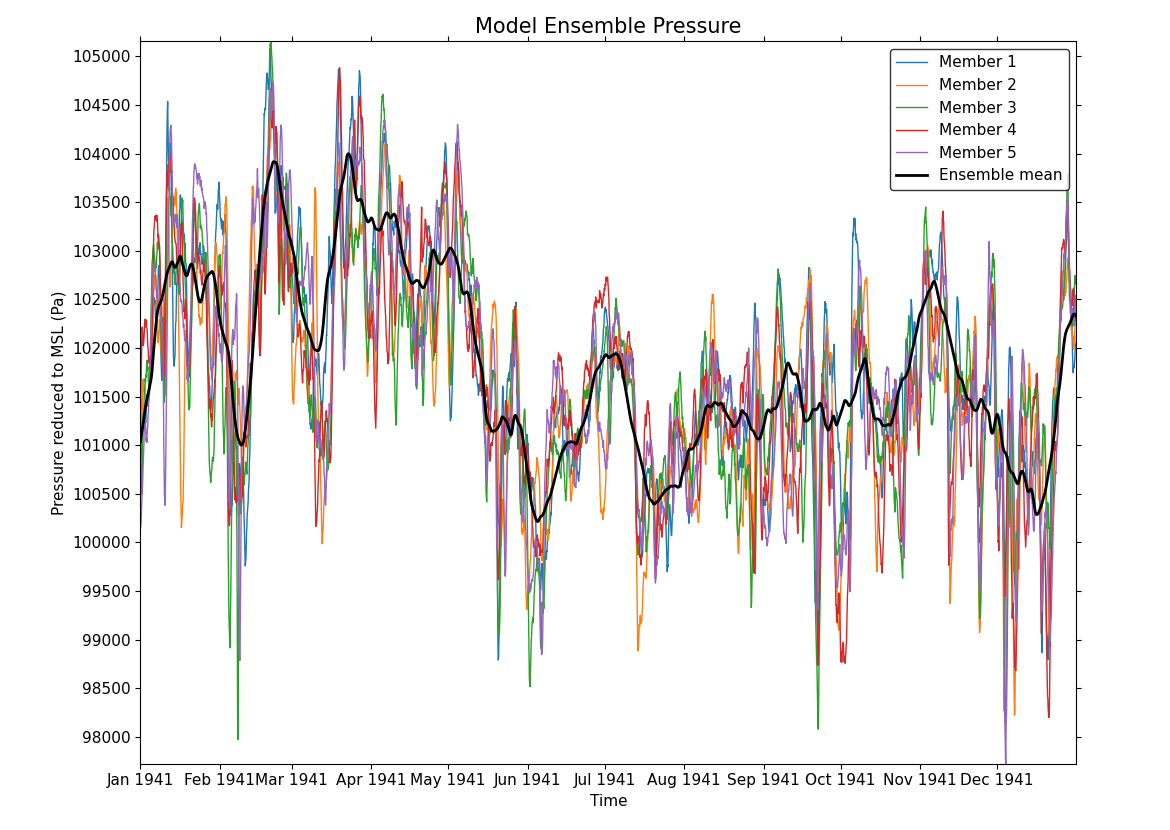
6. Loop over the realizations in the ensemble using the range function and the domain_axis to determine the size of the realization dimension. For each realization, extract a subspace of the ensemble using the subspace method and the 'id%realization' keyword argument along a specific latitude and longitude and plot the realizations from the 4D field using cfplot.lineplot.
A moving average of the ensemble along the time axis, with a window size of 90 (i.e. an approximately 3-month moving average) is calculated using the moving_window method. The mode='nearest' parameter is used to specify how to pad the data outside of the time range. The squeeze method removes any dimensions of size 1 from the field to produce a 2D field:
cfp.gopen()

for realization in range(1, ensemble.domain_axis("id%realization").size + 1):
    cfp.lineplot(
        ensemble.subspace(
            **{"id%realization": realization}, latitude=[0], longitude=[0]
        ).squeeze(),
        label=f"Member {realization}",
        linewidth=1.0,
    )

cfp.lineplot(
    ensemble.moving_window(
        method="mean", window_size=90, axis="T", mode="nearest"
    )[0, :, 0, 0].squeeze(),
    label="Ensemble mean",
    linewidth=2.0,
    color="black",
    title="Model Ensemble Pressure",
)

cfp.gclose()
Total running time of the script: ( 1 minutes 4.205 seconds)