Resampling Land Use Flags to a Coarser Grid

In this recipe, we will compare the land use distribution in different countries using a land use data file and visualize the data as a histogram. This will help to understand the proportion of different land use categories in each country.

The land use data is initially available at a high spatial resolution of approximately 100 m, with several flags defined with numbers representing the type of land use. Regridding the data to a coarser resolution of approximately 25 km would incorrectly represent the flags on the new grids.

To avoid this, we will resample the data to the coarser resolution by aggregating the data within predefined spatial regions or bins. This approach will give a dataset where each 25 km grid cell contains a histogram of land use flags, as determined by the original 100 m resolution data. It retains the original spatial extent of the data while reducing its spatial complexity. Regridding, on the other hand, involves interpolating the data onto a new grid, which can introduce artifacts and distortions in the data.

import cartopy.io.shapereader as shpreader
import matplotlib.pyplot as plt
import numpy as np

1. Import the required libraries. We will use Cartopy’s shapereader to work with shapefiles that define country boundaries:

import cf

2. Read and select land use data by index and see properties of all construcs:

f = cf.read("~/recipes/output.tif.nc")[0]
f.dump()

-------------------------------------------------
Field: long_name=GDAL Band Number 1 (ncvar%Band1)
-------------------------------------------------
Conventions = 'CF-1.5'
GDAL = 'GDAL 3.1.4, released 2020/10/20'
GDAL_AREA_OR_POINT = 'Area'
GDAL_DataType = 'Thematic'
RepresentationType = 'THEMATIC'
_FillValue = -128
_Unsigned = 'true'
history = 'Mon Aug 14 15:57:58 2023: GDAL CreateCopy( output.tif.nc, ... )'
long_name = 'GDAL Band Number 1'
valid_range = array([  0, 255], dtype=int16)

Data(latitude(37778), longitude(101055)) = [[0, ..., 0]]

Domain Axis: latitude(37778)
Domain Axis: longitude(101055)

Dimension coordinate: latitude
    long_name = 'latitude'
    standard_name = 'latitude'
    units = 'degrees_north'
    Data(latitude(37778)) = [24.285323229852995, ..., 72.66262936728634] degrees_north

Dimension coordinate: longitude
    long_name = 'longitude'
    standard_name = 'longitude'
    units = 'degrees_east'
    Data(longitude(101055)) = [-56.50450160064635, ..., 72.90546463309875] degrees_east

Coordinate reference: grid_mapping_name:latitude_longitude
    Coordinate conversion:GeoTransform = -56.50514190170437 0.001280602116034448 0 72.66326966834436 0 -0.001280602116034448
    Coordinate conversion:grid_mapping_name = latitude_longitude
    Coordinate conversion:long_name = CRS definition
    Coordinate conversion:spatial_ref = GEOGCS["WGS 84",DATUM["WGS_1984",SPHEROID["WGS 84",6378137,298.257223563,AUTHORITY["EPSG","7030"]],AUTHORITY["EPSG","6326"]],PRIMEM["Greenwich",0],UNIT["degree",0.0174532925199433,AUTHORITY["EPSG","9122"]],AXIS["Latitude",NORTH],AXIS["Longitude",EAST],AUTHORITY["EPSG","4326"]]
    Datum:inverse_flattening = 298.257223563
    Datum:longitude_of_prime_meridian = 0.0
    Datum:semi_major_axis = 6378137.0
    Dimension Coordinate: longitude
    Dimension Coordinate: latitude

3. Define a function to extract data for a specific country:

• The extract_data function is defined to extract land use data for a specific country, specified by the country_name parameter.

• It uses the Natural Earth shapefile to get the bounding coordinates of the selected country.

• The shpreader.natural_earth function is called to access the Natural Earth shapefile of country boundaries with a resolution of 10 m.

• The shpreader.Reader function reads the shapefile, and the selected country’s record is retrieved by filtering the records based on the NAME_LONG attribute.

• The bounding coordinates are extracted using the bounds attribute of the selected country record.

• The land use data file is then read and subset using these bounding coordinates with the help of the subspace function. The subset data is stored in the f variable.

def extract_data(country_name):
    shpfilename = shpreader.natural_earth(
        resolution="10m", category="cultural", name="admin_0_countries"
    )
    reader = shpreader.Reader(shpfilename)
    country = [
        country
        for country in reader.records()
        if country.attributes["NAME_LONG"] == country_name
    ][0]
    lon_min, lat_min, lon_max, lat_max = country.bounds

    f = cf.read("~/recipes/output.tif.nc")[0]
    f = f.subspace(X=cf.wi(lon_min, lon_max), Y=cf.wi(lat_min, lat_max))

    return f

4. Define a function to plot a histogram of land use distribution for a specific country:

• The digitize function of the cf.Field object is called to convert the land use data into indices of bins. It takes an array of bins (defined by the np.linspace function) and the return_bins=True parameter, which returns the actual bin values along with the digitized data.

• The np.linspace function is used to create an array of evenly spaced bin edges from 0 to 50, with 51 total values. This creates bins of width 1.

• The digitized variable contains the bin indices for each data point, while the bins variable contains the actual bin values.

• The cf.histogram function is called on the digitized data to create a histogram. This function returns a field object with the histogram data.

• The squeeze function applied to the histogram array extracts the histogram data as a NumPy array and removes any single dimensions.

• The total_valid_sub_cells variable calculates the total number of valid subcells (non-missing data points) by summing the histogram data.

• The last element of the bin_counts array is removed with slicing (bin_counts[:-1]) to match the length of the bin_indices array.

• The percentages variable calculates the percentage of each bin by dividing the bin_counts by the total_valid_sub_cells and multiplying by 100.

• The bin_indices variable calculates the center of each bin by averaging the bin edges. This is done by adding the bins.array[:-1, 0] and bins.array[1:, 0] arrays and dividing by 2.

• The ax.bar function is called to plot the histogram as a bar chart on the provided axis. The x-axis values are given by the bin_indices array, and the y-axis values are given by the percentages array.

• The title, x-axis label, y-axis label, and axis limits are set based on the input parameters.

def plot_histogram(field, ax, label, ylim, xlim):
    digitized, bins = field.digitize(np.linspace(0, 50, 51), return_bins=True)

    h = cf.histogram(digitized)
    bin_counts = h.array.squeeze()

    total_valid_sub_cells = bin_counts.sum()

    bin_counts = bin_counts[:-1]

    percentages = bin_counts / total_valid_sub_cells * 100

    bin_indices = (bins.array[:-1, 0] + bins.array[1:, 0]) / 2

    ax.bar(bin_indices, percentages, label=label)
    ax.set_title(label)
    ax.set_xlabel("Land Use Flag")
    ax.set_ylabel("Percentage")
    ax.set_ylim(ylim)
    ax.set_xlim(xlim)

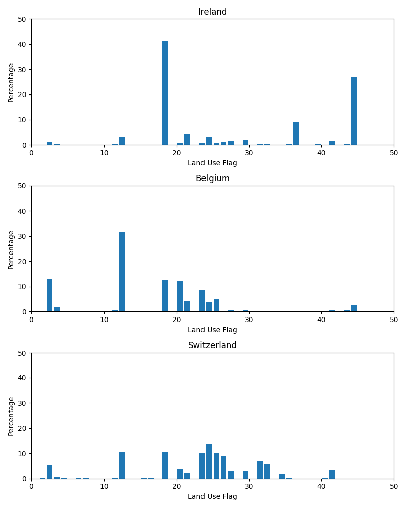
5. Define the countries of interest:

countries = ["Ireland", "Belgium", "Switzerland"]

6. Set up the figure and axes for plotting the histograms:

• The plt.subplots function is called to set up a figure with three subplots, with a figure size of 8 inches by 10 inches.

• A loop iterates over each country in the countries list and for each country, the extract_data function is called to extract its land use data.

• The plot_histogram function is then called to plot the histogram of land use distribution on the corresponding subplot.

• The plt.tight_layout function is called to ensure that the subplots are properly spaced within the figure and finally, the plt.show function displays the figure with the histograms.

fig, axs = plt.subplots(3, 1, figsize=(8, 10))

for i, country in enumerate(countries):
    ax = axs[i]
    data = extract_data(country)
    plot_histogram(data, ax, label=country, ylim=(0, 50), xlim=(0, 50))

plt.tight_layout()
plt.show()