Note
Click here to download the full example code
Plotting global mean temperatures spatially
In this recipe, we will plot the global mean temperature spatially.
Import cf-python and cf-plot:
import cfplot as cfp

import cf
Read the field constructs:
[<CF Field: ncvar%stn(long_name=time(1452), long_name=latitude(360), long_name=longitude(720))>,
 <CF Field: long_name=near-surface temperature(long_name=time(1452), long_name=latitude(360), long_name=longitude(720)) degrees Celsius>]
Select near surface temperature by index and look at its contents:
Field: long_name=near-surface temperature (ncvar%tmp)
-----------------------------------------------------
Data            : long_name=near-surface temperature(long_name=time(1452), long_name=latitude(360), long_name=longitude(720)) degrees Celsius
Dimension coords: long_name=time(1452) = [1901-01-16 00:00:00, ..., 2021-12-16 00:00:00] gregorian
                : long_name=latitude(360) = [-89.75, ..., 89.75] degrees_north
                : long_name=longitude(720) = [-179.75, ..., 179.75] degrees_east
Average the monthly mean surface temperature values by the time axis using the collapse method:
global_avg = temp.collapse("mean", axes="long_name=time")
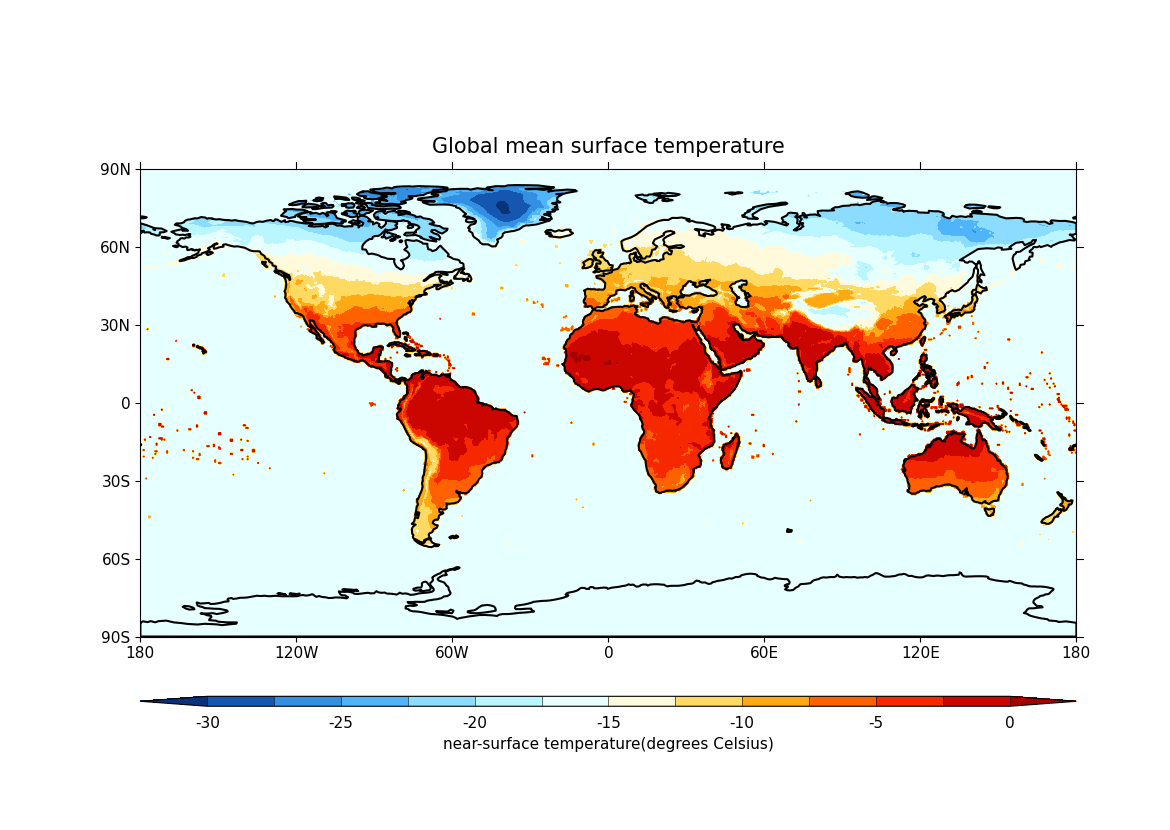
Plot the global mean surface temperatures:
cfp.con(global_avg, lines=False, title="Global mean surface temperature")
Total running time of the script: ( 0 minutes 6.806 seconds)