Calculating and plotting the divergence of sea currents

In this recipe, we will calculate the divergence of depth-averaged currents in the Irish Sea, then plot the divergence as a contour fill plot underneath the vectors themselves in the form of a vector plot.

1. Import cf-python and cf-plot:

import cfplot as cfp

import cf

2. Read the fields in. This dataset consists of depth-averaged eastward and northward current components plus the sea surface height above sea level and is a gridded dataset, with grid resolution of 1.85 km, covering the entire Irish Sea area. It was found via the CEDA Archive at the location of: https://catalogue.ceda.ac.uk/uuid/1b89e025eedd49e8976ee0721ec6e9b5, with DOI of https://dx.doi.org/10.5285/031e7ca1-9710-280d-e063-6c86abc014a0:

f = cf.read("~/recipes/POLCOMS_WAM_ZUV_01_16012006.nc")

3. Get the separate vector components, which are stored as separate fields. The first, ‘u’, corresponds to the eastward component and the second, ‘v’, the northward component:

u = f[0]
v = f[1]

4. Squeeze the fields to remove the size 1 axes in each case:

u = u.squeeze()
v = v.squeeze()

5. Consider the currents at a set point in time. To do this we select one of the 720 datetime sample points in the fields to investigate, in this case by subspacing to pick out a particular datetime value we saw within the time coordinate data of the field (but you could also use indexing or filtering to select a specific value). Once we subspace to one datetime, we squeeze out the size 1 time axis in each case:

chosen_time = "2006-01-15 23:30:00"  # 720 choices to pick from, try this one!
u_1 = u.subspace(T=cf.dt(chosen_time))
v_1 = v.subspace(T=cf.dt(chosen_time))
u_1 = u_1.squeeze()
v_1 = v_1.squeeze()

6. When inspecting the u and v fields using cf inspection methods such as from print(u_1.data) and u_1.data.dump(), for example, we can see that there are lots of -9999 values in their data array, apparently used as a fill/placeholder value, including to indicate undefined data over the land. In order for these to not skew the data and dominate the plot, we need to mask values matching this, so that only meaningful values remain.

u_2 = u_1.where(cf.lt(-9000), cf.masked)
v_2 = v_1.where(cf.lt(-9000), cf.masked)

7. Calculate the divergence using the ‘div_xy’ function operating on the vector eastward and northward components as the first and second argument respectively. We need to calculate this for the latitude-longitude plane of the Earth, defined in spherical polar coordinates, so we must specify the Earth’s radius for the appropriate calculation:

div = cf.div_xy(u_2, v_2, radius="earth")

8. First we configure the overall plot by making the map higher resolution, to show the coastlines of the UK and Ireland in greater detail, and changing the colourmap to better reflect the data which can be positive or negative, i.e. has 0 as the ‘middle’ value of significance, so should use a diverging colour map.

cfp.mapset(resolution="10m")
cfp.cscale("ncl_default", ncols=21)

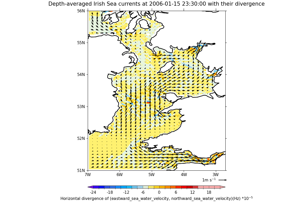
9. Now generate the final plot. Plot the current vectors, noting we had to play around with the ‘stride’ and ‘scale’ parameter values to adjust the vector spacing and size so that the vector field is best represented and visible without over-cluttering the plot. Finally we plot the divergence as a contour plot without any lines showing. This compound plot is saved on one canvas using ‘gopen’ and ‘gclose’ to wrap the two plotting calls:

cfp.gopen()
cfp.vect(u=u_2, v=v_2, stride=6, scale=3, key_length=1)
cfp.con(
    div,
    lines=False,
    title=(
        f"Depth-averaged Irish Sea currents at {chosen_time} with "
        "their divergence"
    ),
)
cfp.gclose()