Note
Click here to download the full example code
Using mask to plot Aerosol Optical Depth
In this recipe, we will make use of a masked array to plot the high-quality retrieval of Aerosol Optical Depth (AOD) from all other retrievals.
Import cf-python, cf-plot and matplotlib.pyplot:
import cfplot as cfp
import matplotlib.pyplot as plt

import cf
Read the field constructs:
[<CF Field: long_name=AOT at 0.55 micron for both ocean and land(ncdim%Rows(768), ncdim%Columns(3200)) 1>,
 <CF Field: long_name=Retrieval AOD550 for each land aerosol model: dust, generic, urban, smoke(ncdim%Rows(768), ncdim%Columns(3200), ncdim%LndLUTnchn(4)) 1>,
 <CF Field: long_name=AOT at 5 ABI channels (0.47, 0.64, 0.86, 1.61, 2.26 microns)(ncdim%Rows(768), ncdim%Columns(3200), ncdim%AbiAODnchn(11)) 1>,
 <CF Field: long_name=Aerosol model: 0-oceanic, 1-dust, 2-generic, 3-urban, 4-heavy smoke(ncdim%Rows(768), ncdim%Columns(3200)) 1>,
 <CF Field: long_name=Angstrom Exponent for 0.55 and 0.86 micron(ncdim%Rows(768), ncdim%Columns(3200)) 1>,
 <CF Field: long_name=Angstrom Exponent for 0.86 and 1.61 micron(ncdim%Rows(768), ncdim%Columns(3200)) 1>,
 <CF Field: long_name=Cloud Mask Quality Flag(ncdim%Rows(768), ncdim%Columns(3200)) 1>,
 <CF Field: long_name=Retrieved coarse aerosol model index over ocean(ncdim%Rows(768), ncdim%Columns(3200)) 1>,
 <CF Field: long_name=Retrieved fine aerosol model index over ocean(ncdim%Rows(768), ncdim%Columns(3200)) 1>,
 <CF Field: long_name=Retrieved ratio of fine mode optical depth at 0.55 micron over ocean(ncdim%Rows(768), ncdim%Columns(3200)) 1>,
 <CF Field: long_name=Percent of high quality retrievals %>,
 <CF Field: long_name=Mean AOD at 550 nm %>,
 <CF Field: long_name=Mean High Quality AOD at 550 nm %>,
 <CF Field: long_name=Retrieval quality:  0: high; 1: medium; 2: low; 3: no retrieval(ncdim%Rows(768), ncdim%Columns(3200)) 1>,
 <CF Field: long_name=External flags from input masks: bit 0&1: cloud (0-confClr/1-probClr/2-probCld/3-confCld); bit 2: snow (0-No/1-Yes); bit 3: cloud shadow; bit 4: fire; bit 5: sun glint; bit 6: Heavy aerosol(ncdim%Rows(768), ncdim%Columns(3200)) 1>,
 <CF Field: long_name=Flags for input data (0-valid/1-invalid): bit 0: geolocation;  bit 1: geometry; bit 2: ancillary model data; bit 3: reflectance(ncdim%Rows(768), ncdim%Columns(3200)) 1>,
 <CF Field: long_name=Flags for retrieval path (0-No/1-Yes): bit 0: retrieval over water; bit 1: over bright land; bit 2: over glint water; bit 3: retrieval with SW scheme over land; bit 4: retrieval with SWIR scheme over land; bit 5: retrieval over bright-land algorithm, bit 6: dark land retrieval over bright land(ncdim%Rows(768), ncdim%Columns(3200)) 1>,
 <CF Field: long_name=Flags for retrieval (0-No/1-Yes): bit 0: retrieval failed; bit 1: airmass exceeds threshold; bit 2: dark barren land surface type; bit 3: extrapolation involved; bit 4: retrieval residula out of range; bit 5: dark land NDVI out of range; bit 6: dark land redness ratio out of range; bit 7: adjacent to cloud or snow(ncdim%Rows(768), ncdim%Columns(3200)) 1>,
 <CF Field: long_name=Flags for internal tests (0-No/1-Yes): bit 0: cloudy; bit 1: cirrus; bit 2: thin cirrus; bit 3: inhomogeneous; bit 4: snow/ice; bit 5: ephemeral water; bit 6: shallow water; bit 7: heavy aerosol(ncdim%Rows(768), ncdim%Columns(3200)) 1>,
 <CF Field: long_name=Retrieval residual for each land aerosol model: dust, generic, urban, smoke(ncdim%Rows(768), ncdim%Columns(3200), ncdim%LndLUTnchn(4)) 1>,
 <CF Field: long_name=Retrieval residual of the best solution(ncdim%Rows(768), ncdim%Columns(3200)) 1>,
 <CF Field: long_name=Percent of AOD retrievals %>,
 <CF Field: long_name=land surface reflectance at 0.47, 0.64 and 2.26 micron(ncdim%Rows(768), ncdim%Columns(3200), ncdim%AbiAODnchn(11)) 1>,
 <CF Field: long_name=Inhomogeneity TOA reflectance standard deviation: 0.47 micron over land, 2.26 micron over ocean(ncdim%Rows(768), ncdim%Columns(3200)) 1>,
 <CF Field: long_name=Start column index 1>,
 <CF Field: long_name=Start row index 1>,
 <CF Field: long_name=Cloud Mask Granule Level Degradation Quality Flag 1>]
Select AOD from the field list by identity and look at the contents:
aod = fl.select_field("long_name=AOT at 0.55 micron for both ocean and land")
print(aod)
Field: long_name=AOT at 0.55 micron for both ocean and land (ncvar%AOD550)
--------------------------------------------------------------------------
Data            : long_name=AOT at 0.55 micron for both ocean and land(ncdim%Rows(768), ncdim%Columns(3200)) 1
Auxiliary coords: long_name=Longitude(ncdim%Rows(768), ncdim%Columns(3200)) = [[94.47801971435547, ..., 63.974063873291016]] degrees_east
                : long_name=Latitude(ncdim%Rows(768), ncdim%Columns(3200)) = [[21.498714447021484, ..., 22.031387329101562]] degrees_north
Select AOD retrieval quality by index and look at the quality flags:
Field: long_name=Retrieval quality:  0: high; 1: medium; 2: low; 3: no retrieval (ncvar%QCAll)
----------------------------------------------------------------------------------------------
Data            : long_name=Retrieval quality:  0: high; 1: medium; 2: low; 3: no retrieval(ncdim%Rows(768), ncdim%Columns(3200)) 1
Auxiliary coords: long_name=Longitude(ncdim%Rows(768), ncdim%Columns(3200)) = [[94.47801971435547, ..., 63.974063873291016]] degrees_east
                : long_name=Latitude(ncdim%Rows(768), ncdim%Columns(3200)) = [[21.498714447021484, ..., 22.031387329101562]] degrees_north
5. Select latitude and longitude dimensions by identities, with two different techniques:
lon = aod.coordinate("long_name=Longitude")
lat = aod.coordinate("Y")
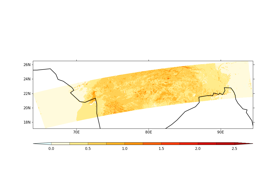
6. Plot the AOD for all the retrievals using
cfplot.con. Here the argument
'ptype' specifies the type of plot to use (latituide-longitude here) and
the argument 'lines=False' does not draw contour lines:
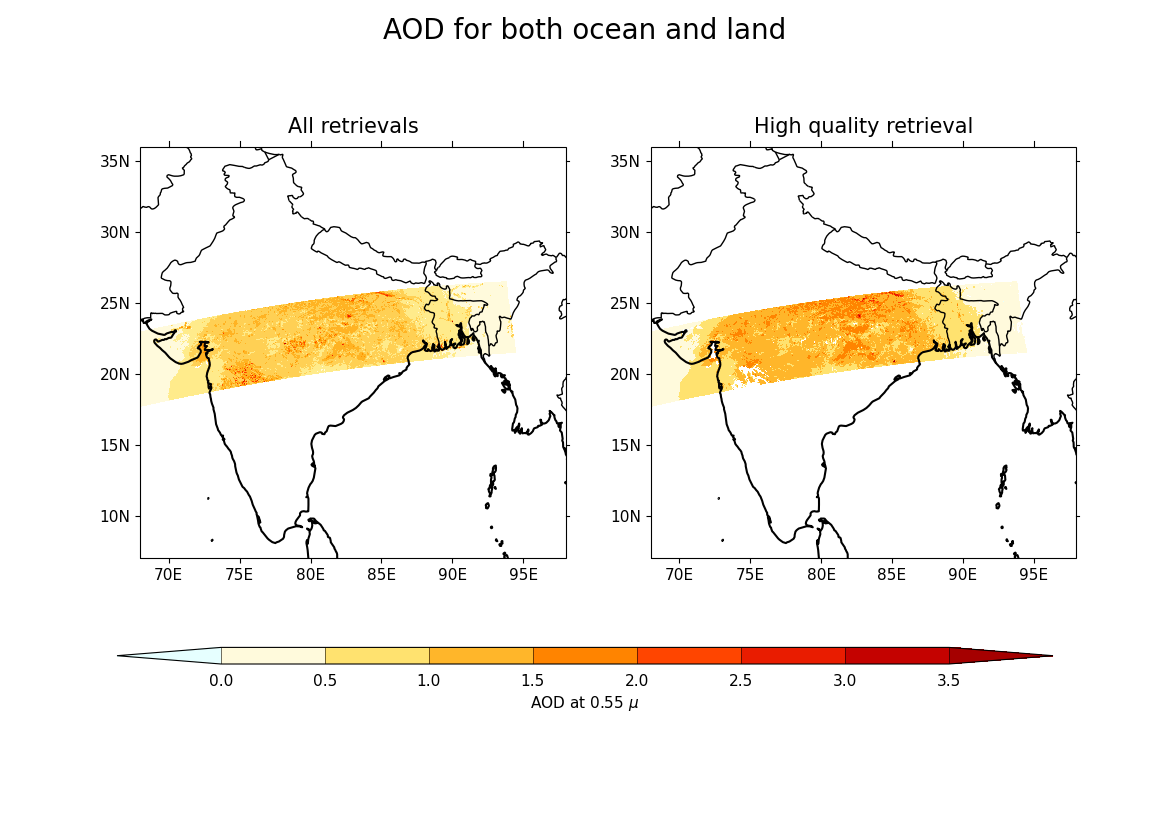
7. Create a mask for AOD based on the quality of the retrieval. The
'__ne__' method is an implementation of the != operator. It is used to
create a mask where all the high-quality AOD points (with the flag 0) are
marked as False, and all the other data points (medium quality, low
quality, or no retrieval) are marked as True:
8. Apply the mask to the AOD dataset. The 'where' function takes the
mask as an input and replaces all the values in the AOD dataset that
correspond to True in the mask with a masked value using cf.masked.
In this case, all AOD values that are not of high-quality (since they were
marked as True in the mask) are masked. This means that the high
variable contains only the AOD data that was retrieved with high-quality:
9. Now plot both the AOD from high-quality retrieval and all other retrievals using cfplot.con. Here:
cfplot.gopen is used to define the parts of the plot area, specifying that the figure should have 1 row and 2 columns, which is closed by cfplot.gclose;
plt.suptitle is used to add a title for the whole figure;
the subplots for plotting are selected using cfplot.gpos after which cfplot.mapset is used to set the map limits and resolution for the subplots;
and as cf-plot stores the plot in a plot object with the name
cfp.plotvars.plot, country borders are added using normal Cartopy operations on thecfp.plotvars.mymapobject:
import cartopy.feature as cfeature

cfp.gopen(rows=1, columns=2, bottom=0.2)
plt.suptitle("AOD for both ocean and land", fontsize=20)
cfp.gpos(1)
cfp.mapset(resolution="50m", lonmin=68, lonmax=98, latmin=7, latmax=36)
cfp.con(
    f=aod.array,
    x=lon.array,
    y=lat.array,
    ptype=1,
    lines=False,
    title="All retrievals",
    colorbar=None,
)
cfp.plotvars.mymap.add_feature(cfeature.BORDERS)
cfp.gpos(2)
cfp.mapset(resolution="50m", lonmin=68, lonmax=98, latmin=7, latmax=36)
cfp.con(
    f=high.array,
    x=lon.array,
    y=lat.array,
    ptype=1,
    lines=False,
    title="High quality retrieval",
    colorbar_position=[0.1, 0.20, 0.8, 0.02],
    colorbar_orientation="horizontal",
    colorbar_title="AOD at 0.55 $\mu$",
)
cfp.plotvars.mymap.add_feature(cfeature.BORDERS)
cfp.gclose()
Total running time of the script: ( 1 minutes 2.707 seconds)