Multiple plots

Example 19a: Multiple plots

Making a single figure with multiple plots on it

f = cf.read(f"cfplot_data/ggap.nc")[1]
cfp.gopen(rows=2, columns=2, bottom=0.2)
cfp.gpos(1)
cfp.con(f.subspace(pressure=500), colorbar=None)
cfp.gpos(2)
cfp.mapset(proj="moll")
cfp.con(f.subspace(pressure=500), colorbar=None)
cfp.gpos(3)
cfp.mapset(proj="npstere", boundinglat=30, lon_0=180)
cfp.con(f.subspace(pressure=500), colorbar=None)
cfp.gpos(4)
cfp.mapset(proj="spstere", boundinglat=-30, lon_0=180)
cfp.con(
    f.subspace(pressure=500),
    colorbar_position=[0.1, 0.1, 0.8, 0.02],
    colorbar_orientation="horizontal",
)
cfp.gclose()

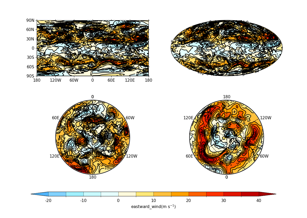
Plots are arranged over rows and columns with the first plot at the top left and the last plot is the bottom right. Here the margin at the bottom of the plot is increased with the bottom parameter to gopen to accomodate a unified colorbar. The colorbars are turned off for all plots apart from the last one.

Example 19b: Multiple plots with user-specified plot positions

Making a single figure with multiple plots on it, where the positions of the individual plots are set explicitly

f = cf.read(f"cfplot_data/ggap.nc")[1]

cfp.gopen(user_position=True)

cfp.gpos(xmin=0.1, xmax=0.5, ymin=0.55, ymax=1.0)
cfp.con(f.subspace(Z=500), title="500mb", lines=False)

cfp.gpos(xmin=0.55, xmax=0.95, ymin=0.55, ymax=1.0)
cfp.con(f.subspace(Z=100), title="100mb", lines=False)

cfp.gpos(xmin=0.3, xmax=0.7, ymin=0.1, ymax=0.55)
cfp.con(f.subspace(Z=10), title="10mb", lines=False)

cfp.gclose()

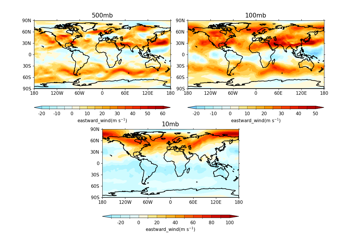
User specified plot limits are set by first specifying the user_position=True parameter to gopen and then the plot position to the gpos routines. The xmin, xmax, ymin, ymax paramenters for the plot display area are in normalised coordinates.

Cylidrical projection plots have an additional rider of having a degree in longitude and latitude being the same size so plots of this type might not fill the plot area specified as expected.

Example 19c: Accomodating more than one colour bar

Using the approach to make a single figure with multiple plots on it to fit an extra colour bar

f = cf.read(f"cfplot_data/ggap.nc")[1]
g = f.collapse("X: mean")

cfp.gopen(user_position=True)

cfp.gpos(xmin=0.2, ymin=0.2, xmax=0.8, ymax=0.8)
cfp.lineplot(
    g.subspace(pressure=100),
    marker="o",
    color="blue",
    title="Zonal mean zonal wind at 100mb",
)

cfp.cscale("seaice_2", ncols=20)
levs = np.arange(282, 320, 2)
cfp.cbar(levs=levs, position=[0.2, 0.1, 0.6, 0.02], title="seaice_2")

cfp.cscale("topo_15lev", ncols=22)
levs = np.arange(-100, 2000, 100)
cfp.cbar(
    levs=levs,
    position=[0.03, 0.2, 0.04, 0.6],
    orientation="vertical",
    title="topo_15lev",
)

cfp.gclose()

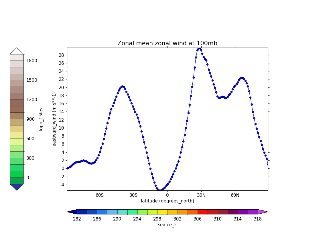
The plot position on the page is set manually with the user_position=True parameter to cfp.gopen and then passing the required plot size to cfp.gpos. Two calls to the cfp.cbar routine place colour bars on the plot.