Rotated pole plots#

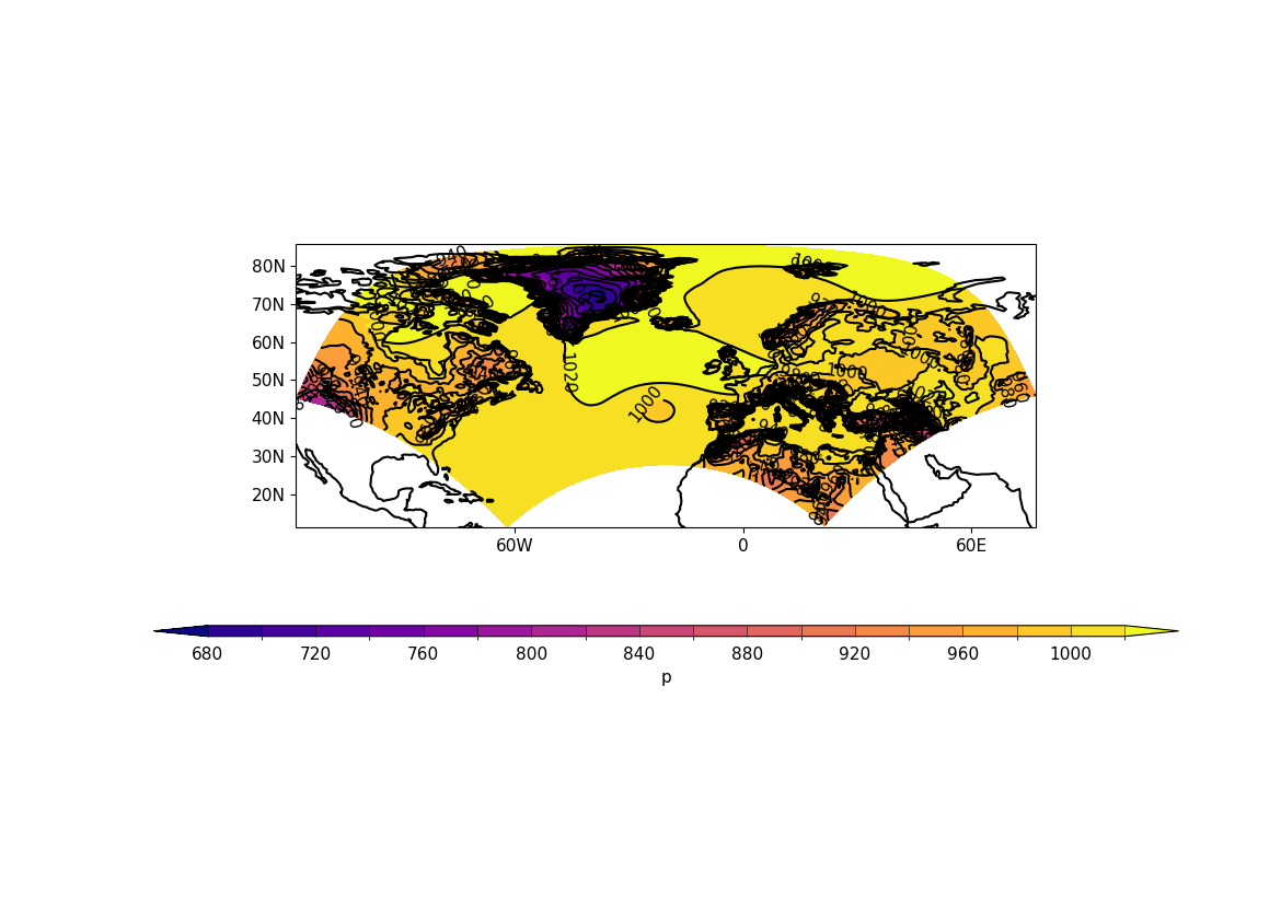
Example 21b: Plot of rotated pole data#

Making a plot of data defined on a rotated pole coordinate system#

f = cf.read(f"cfplot_data/rgp.nc")[0]

cfp.cscale("plasma")

cfp.con(f)

Example 22: Plot of rotated pole data on its native grid#

Making a plot of data defined on a rotated pole coordinate system shown on its native grid#

f = cf.read(f"cfplot_data/rgp.nc")[0]

cfp.cscale("plasma")
cfp.mapset(proj="rotated")

cfp.con(f)

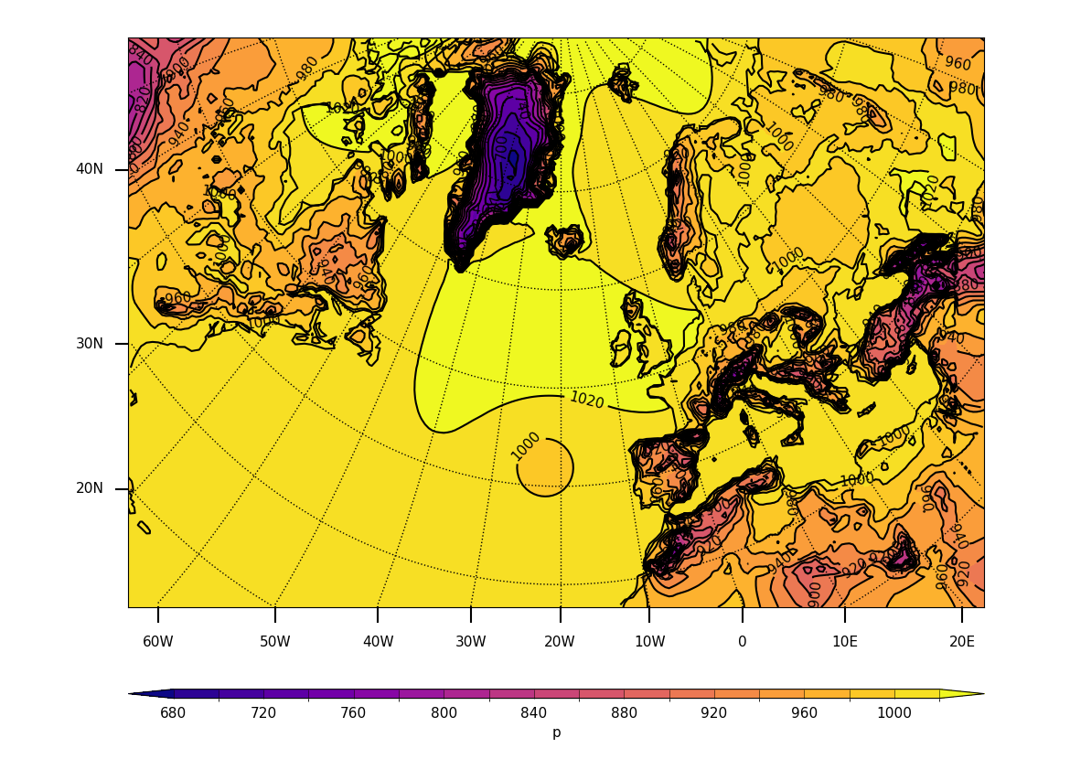
This plot shows some rotated pole data on the native grid. Notice the way that the longitude lines are warped away from the centre of the plot. Data over the equatorial regions show little of this warping.

Example 23b: Overlaying vectors over a rotated pole data plot#

TODO describe Example 23 Other#

f = cf.read(
    f"cfplot_data/20160601-05T0000Z_INCOMPASS_km4p4_uv_RH_500.nc"
)
cfp.mapset(50, 100, 5, 35)
cfp.levs(0, 90, 15, extend="neither")

cfp.gopen()
cfp.con(f[0], lines=False)
cfp.vect(u=f[1], v=f[2], stride=40, key_length=10)
cfp.gclose()

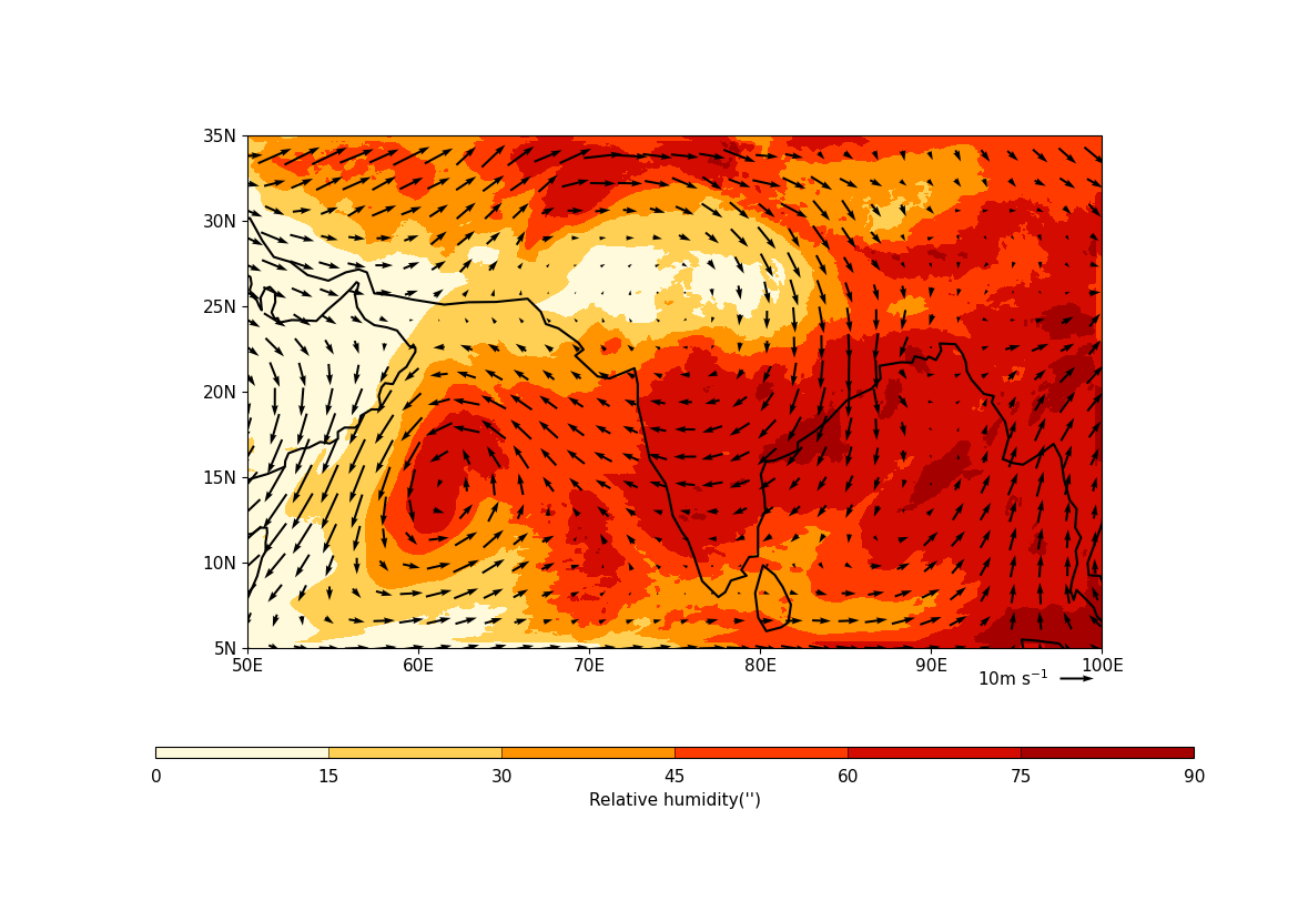
In this plot a cylindrical projection plot of rotated pole data is overlayed with wind vectors.

Care is needed when making vector plots as the vectors can be of two forms:
a) eastward wind and westward wind are relative to longitude and
latitude axes
b) x-wind and y-wind are relative to the rotated pole axes

Here we have eastward and westward wind so these can be plotted as normal over a cylindrical projection. For the case of data in case b) above, the x-wind and y-wind will need to be appropriately rotated onto a cylindrical grid.

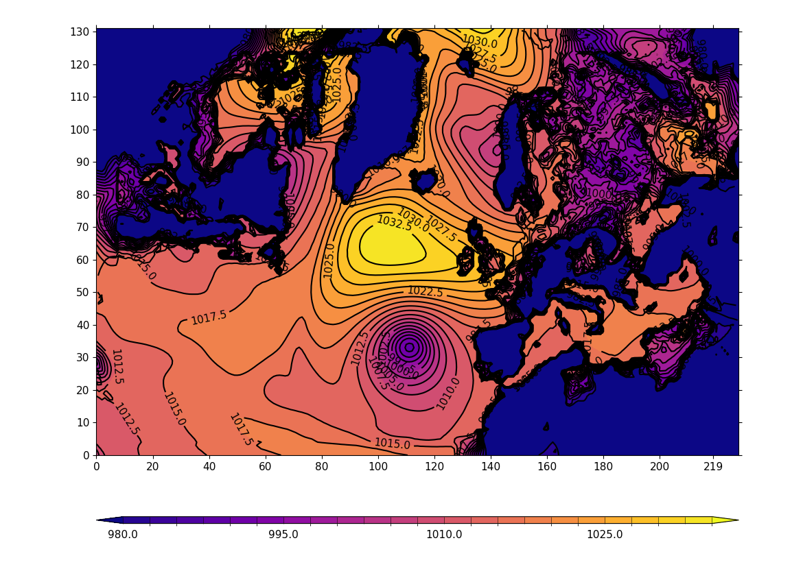
Example 23a: Rotated pole plot from data which is not CF Compliant#

Constructing a rotated pole plot from data which is not very CF Compliant, noting that this takes more set up than for CF Compliant data (see Example 21b)#

f = cf.read(f"cfplot_data/rgp.nc")[0]

data = f.array
xvec = f.construct("ncvar%x").array
yvec = f.construct("ncvar%y").array
xpole = 160
ypole = 30

cfp.gopen()
cfp.cscale("plasma")
xpts = np.arange(np.size(xvec))
ypts = np.arange(np.size(yvec))
cfp.gset(
    xmin=0, xmax=np.size(xvec) - 1, ymin=0, ymax=np.size(yvec) - 1
)
cfp.levs(min=980, max=1035, step=2.5)
cfp.con(data, xpts, ypts[::-1])
cfp.rgaxes(xpole=xpole, ypole=ypole, xvec=xvec, yvec=yvec)
cfp.gclose()