Examples

Below is a gallery showcasing particular examples introducing a type/theme category, but to browse all examples please consult the full listing.

Gallery

In this gallery one particular example is highlighted to illustrate each type/theme category, but you are encouraged to explore further examples by clicking through to the category pages.

Contour plots

cylindrical.html#example-1-basic-contour-plot-in-default-projection

Blockfill plots

cylindrical.html#example-2-basic-blockfill-plot-in-default-projection

Vector plots

vectors.html#example-13-basic-vector-plot

Stream plots

vectors.html#example-16c-stream-plot-in-a-colour-scale

Stipple plots

stipple_plots.html#example-17-basic-stipple-plot

Trajectories

trajectories.html#example-42b-tracks-displayed-in-a-colour-scale

Hovmöller plots

hovmuller.html#example-11-latitude-time-subset-view-hovmoller-plot

Vertical (pressure or height) plots

pressure.html#example-8-latitude-against-log-of-pressure-over-longitude-zonal-mean

Lineplots

graphs.html#example-27-basic-line-plot

Support for multiple projections

projections.html#example-34-cropping-the-lambert-conformal-conic-lcc-projection

Polar projection views

trajectories.html#example-40-tracks-in-the-polar-stereographic-projection

Unstructured grids (UGRID) support

unstructured.html#example-24a-ugrid-blockfill-plot-with-lfric-cubed-sphere-mesh-output

Rotated pole support

rotated_pole.html#example-22-plot-of-rotated-pole-data-on-its-native-grid

Multiple plots on one figure

multiple_plots.html#example-19b-multiple-plots-with-user-specified-plot-positions

Flexible customisation e.g. user-defined axes

user_defined.html#example-21a-user-defined-axes

Listing of all examples

Note

All example code assumes the following imports have been made, where numpy is usually not required but it is for some of the examples:

Imports required as setup for the examples, noting that cfplot is always aliased to cfp by convention

import cfplot as cfp
import cf
import numpy as np  # only required for some examples

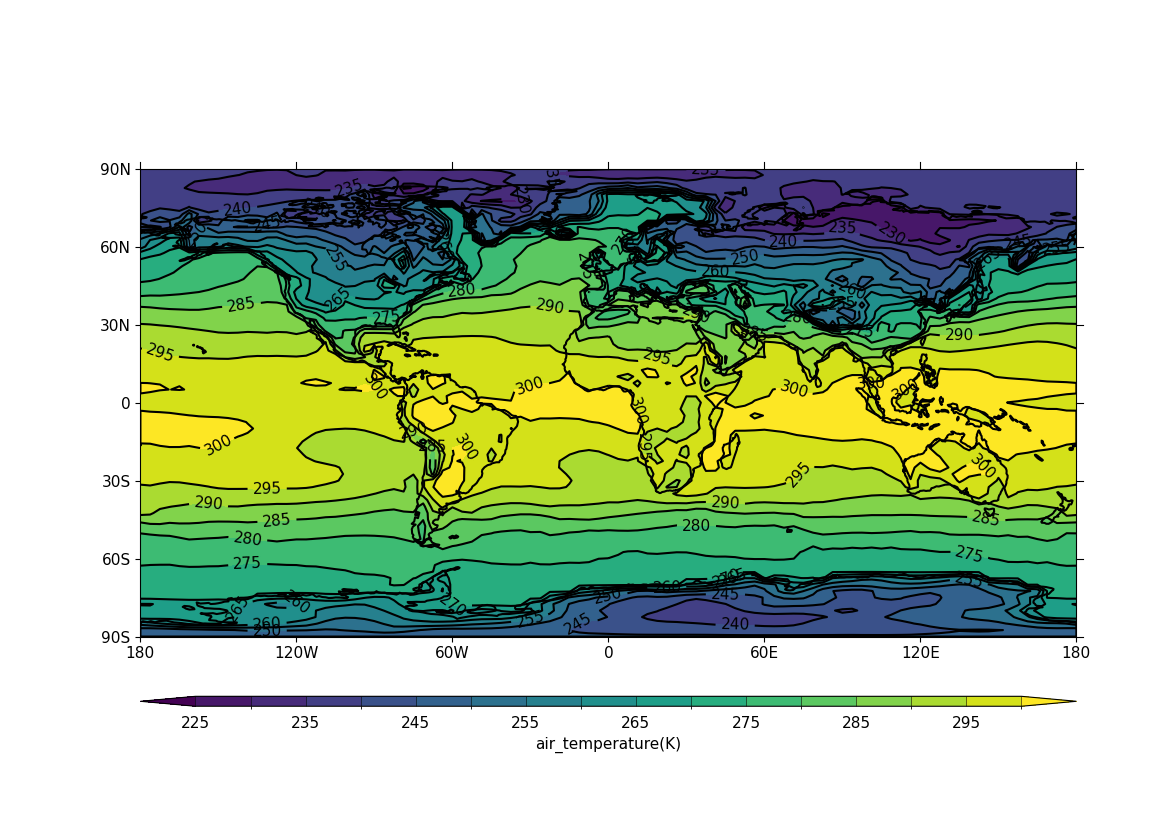
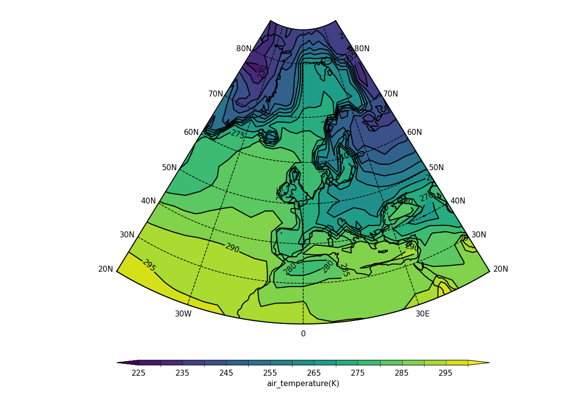
• Example 1: Basic contour plot in default projection
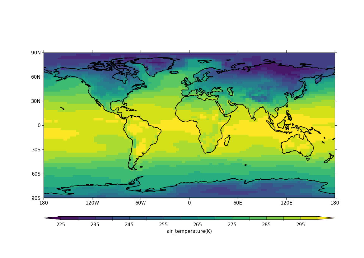
• Example 2: Basic blockfill plot in default projection
• Example 3: Contour plot with altered map limits and levels
• Example 4: North Pole polar stereographic projection contour plot
• Example 5: South Pole polar projection contour plot with bounding latitude
• Example 6: Latitude-pressure plot at set longitude
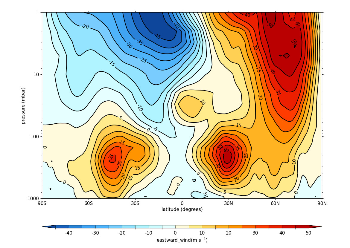
• Example 7: Latitude-pressure plot over zonal mean
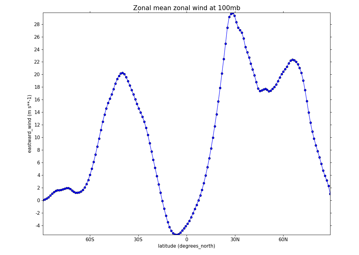
• Example 8: Latitude against log of pressure over longitude zonal mean
• Example 9: Longitude-pressure plot over latitude mean
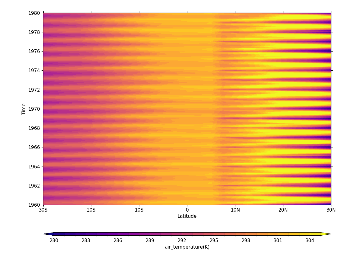
• Example 10: Latitude-time Hovmöller plot
• Example 11: Latitude-time subset view Hovmöller plot
• Example 12: Longitude-time Hovmöller plot
• Example 13: Basic vector plot
• Example 14: Vector plot overlaid on a contour map
• Example 15: Polar projection vector plot
• Example 16a: Zonal vector plot
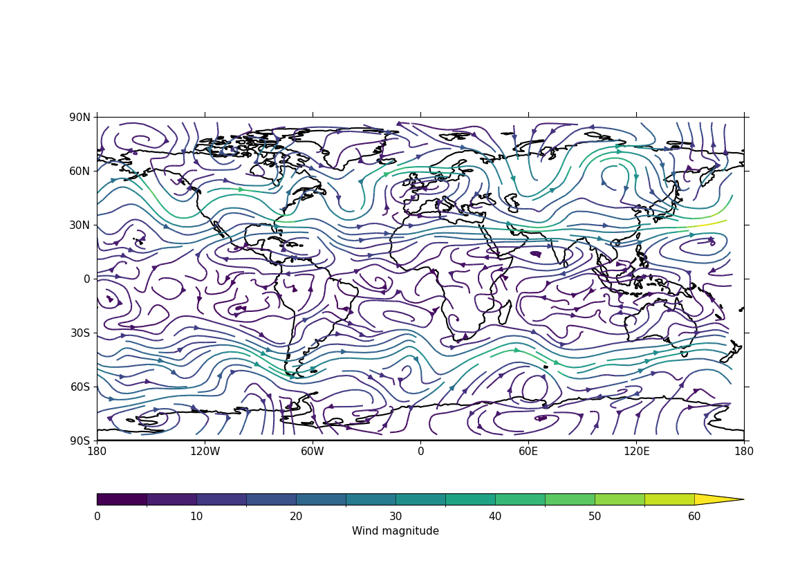
• Example 16b: Basic stream plot
• Example 16c: Stream plot in a colour scale
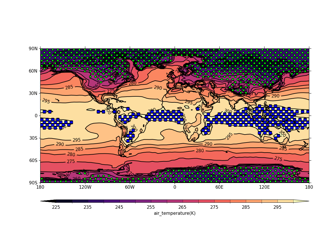
• Example 17: Basic stipple plot
• Example 18: Polar stipple plot
• Example 19a: Multiple plots
• Example 19b: Multiple plots with user-specified plot positions
• Example 19c: Accomodating more than one colour bar
• Example 20: Case where user-defined axis labels are required
• Example 21a: User-defined axes
• Example 21b: Plot of rotated pole data
• Example 22: Plot of rotated pole data on its native grid
• Example 23a: Rotated pole plot from data which is not CF Compliant
• Example 23b: Overlaying vectors over a rotated pole data plot
• Example 24a: UGRID blockfill plot with LFRic cubed sphere mesh output
• Example 24b: UGRID plot in the polar stereographic projection view
• Example 25: UGRID contour plot with ORCA 2 output
• Example 26a: Contour plot based on discrete feature values
• Example 26b: Contour plot from discrete feature values with labelling
• Example 27: Basic line plot
• Example 28: Line plot with a legend
• Example 29: Time series line plot
• Example 30: Line plot with two x axes
• Example 31: UKCP projection
• Example 32: UKCP projection with blockfill
• Example 33: OSGB and EuroPP projections
• Example 34: Cropping the Lambert Conformal Conic (LCC) projection
• Example 35: Mollweide projection
• Example 36: Mercator projection
• Example 37: Orthographic projection
• Example 38: Robinson projection
• Example 39: Basic track plotting
• Example 39b: plotting a single (1D) DSG trajectory
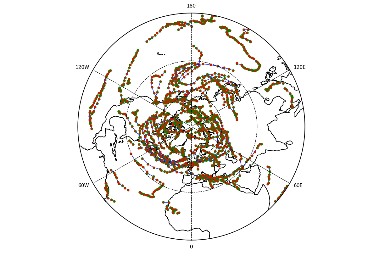
• Example 40: Tracks in the polar stereographic projection
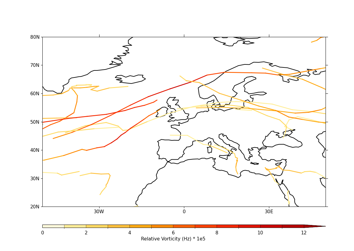
• Example 41: Feature propagation over Europe
• Example 42a: Tracks with labelled data points
• Example 42b: Tracks displayed in a colour scale
• Example 43: CF-compliant WRF model output data

Example Datasets

The examples make use of a small number of sample datasets. These are available to view and download from a dedicated directory in the codebase repository. Alternatively, they may be downloaded together as a pair of zip files (split into two parts to fit within GitHub file size limits, total size ~125 MB) available from here (part 1 of 2) and here (part 2 of 2) which can be unzipped together to the full dataset directory as follows:

Accessing all of the datasets for the cf-plot examples

# Download the split zip parts: either use 'wget' as below or
# download both files from the links above
wget https://github.com/NCAS-CMS/cf-plot/tree/main/docs/source/_downloads/example-datasets.z01
wget https://github.com/NCAS-CMS/cf-plot/tree/main/docs/source/_downloads/example-datasets.zip

# Recombine into a single zip (zip -s0 merges split parts)
zip -s0 example-datasets.zip --out all-example-datasets.zip

# Unzip the merged file
unzip all-example-datasets.zip