Unstructured grids and UGRID#

Unstructured grids have data points in non-regular locations. Examples of these are the LFRic model grid, the ORCA ocean grid and weather station data.

The UGRID Conventions are conventions for storing unstructured (or flexible mesh) model data in netCDF. As of CF-1.11, version 1.0 of UGRID is partially included within the CF Conventions.

This page demonstrates how to plot data in the form of both UGRID-compliant netCDF and NumPy arrays of unstructured data.

Example 24a: UGRID blockfill plot with LFRic cubed sphere mesh output#

Making a blockfill plot of UGRID data, specifically LFRic model output which is defined on a cubed sphere mesh#

f = cf.read("cfplot_data/lfric_initial.nc")

# Select the relevant fields for the objects required for the plot,
# taking the air potential temperature as a variable to choose to view.
pot = f.select_by_identity("air_potential_temperature")[0]
lats = f.select_by_identity("latitude")[0]
lons = f.select_by_identity("longitude")[0]
faces = f.select_by_identity("cf_role=face_edge_connectivity")[0]

# Reduce the variable to match the shapes
pot = pot[4,:]

cfp.levs(240, 310, 5)

cfp.con(
    f=pot, face_lons=lons, face_lats=lats,
    face_connectivity=faces, lines=False, blockfill=True,
)

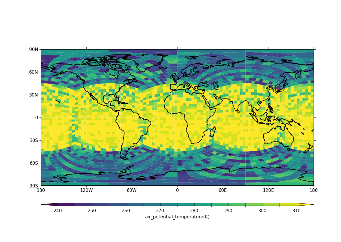
Here we identify the fields in the data that have the longitudes and latitudes for the corner points for the field and pass them to cfp.con. Once UGRID is in the CF metadata conventions the face plotting commands will be simplified as the face connectivity, associated longitudes and latitudes will all be described within the data field. The plotted data is a test field of potential temperature and isn't realistic in regards to the actual values.

Example 24b: UGRID plot in the polar stereographic projection view#

TODO describe Example 24b#

f = cf.read("cfplot_data/lfric_initial.nc")

# Select the relevant fields for the objects required for the plot,
# taking the air potential temperature as a variable to choose to view.
pot = f.select_by_identity("air_potential_temperature")[0]
lats = f.select_by_identity("latitude")[0]
lons = f.select_by_identity("longitude")[0]
faces = f.select_by_identity("cf_role=face_edge_connectivity")[0]

# Reduce the variable to match the shapes
pot = pot[4,:]

cfp.levs(240, 310, 5)

# This time set the projection to a polar one for a different view
cfp.mapset(proj="npstere")
cfp.con(
    f=pot, face_lons=lons,
    face_lats=lats, face_connectivity=faces, lines=False,
    blockfill=True,
)

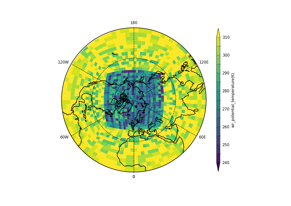
Here the projection was changed to show the north pole.

Example 24c: UGRID contour plot with LFRic cubed sphere mesh output#

Making a contour plot of UGRID data, specifically LFRic model output which is defined on a cubed sphere mesh (see Example 24a for a more effective plot form for this, blockfill)#

f = cf.read("cfplot_data/lfric_initial.nc")
pot = f.select_by_identity("air_potential_temperature")[0]

g = pot[0, :]
cfp.con(g, lines=False)

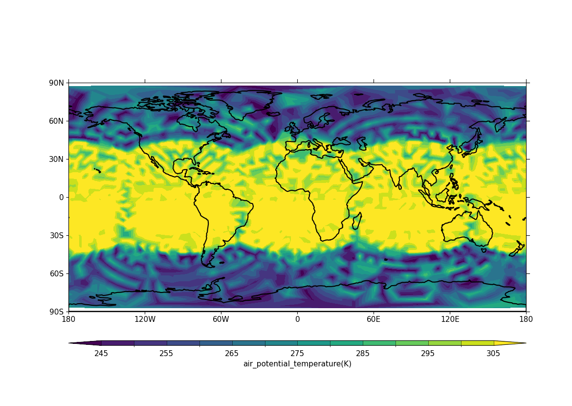
The data in the field has auxiliary longitudes and latitudes that can be contoured as normal. Internally in cf-plot this is made using the matplotlib tricontourf function as the data points are spatially irregular.

Example 25: UGRID contour plot with ORCA 2 output#

Making a contour plot of UGRID data, specifically ORCA 2 ocean-only grid data#

f = cf.read(f"cfplot_data/orca2.nc")

# Get an Orca grid and flatten the arrays
lons = f.select_by_identity("ncvar%longitude")[0]
lats = f.select_by_identity("ncvar%latitude")[0]
temp = f.select_by_identity("ncvar%sst")[0]

lons.flatten(inplace=True)
lats.flatten(inplace=True)
temp.flatten(inplace=True)

# Note: in this case we can't input the 'temp' field as-is,
# because it isn't CF-compliant, notably it doesn't have
# coordinates of any kind set. So we must pull out the array
# and input that, along with the corresponding lat and lon arrays.
cfp.con(f=temp.array, x=lons.array, y=lats.array, ptype=1)

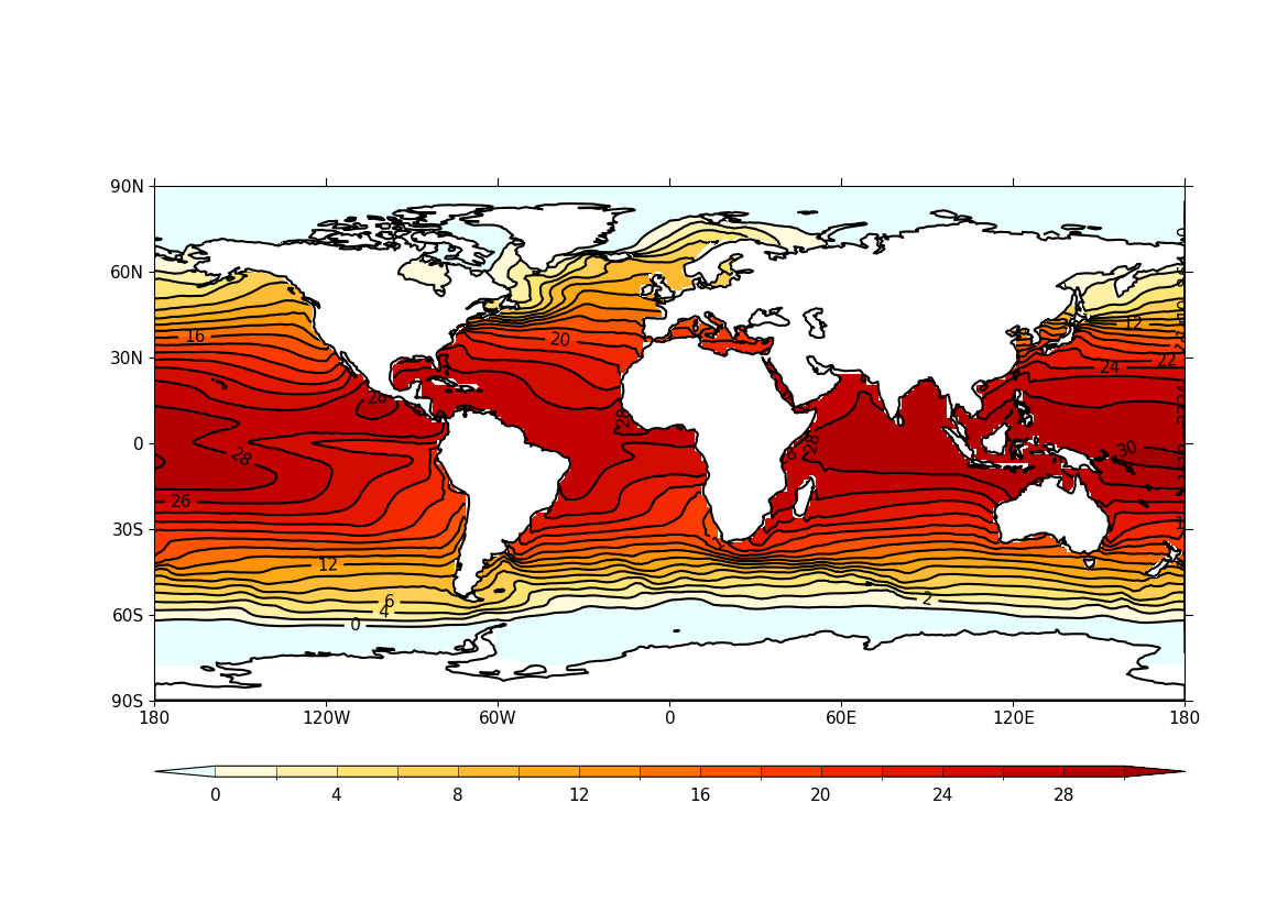
The ORCA2 grid is an ocean grid with missing values over the land points. The data in this file is from before the UGRID convention was started and has no face connectivity or corner coordinates. In this case we can only plot a normal contour plot.

Here we read in temperature data in a text file from meteorological stations around the British Isles and make a contour plot.

Example 26a: Contour plot based on discrete feature values#

Making a contour plot where the contours are determined from discrete feature values, in this case station data#

# Arrays for data
lons = []
lats = []
pressure = []
temp = []

# Read data and make the contour plot
f = open("cfplot_data/synop_data.txt")
lines = f.readlines()
for line in lines:
    mysplit = line.split()
    lons = np.append(lons, float(mysplit[1]))
    lats = np.append(lats, float(mysplit[2]))
    pressure = np.append(pressure, float(mysplit[3]))
    temp = np.append(temp, float(mysplit[4]))

cfp.con(
    x=lons, y=lats, f=temp, ptype=1, colorbar_orientation="vertical"
)

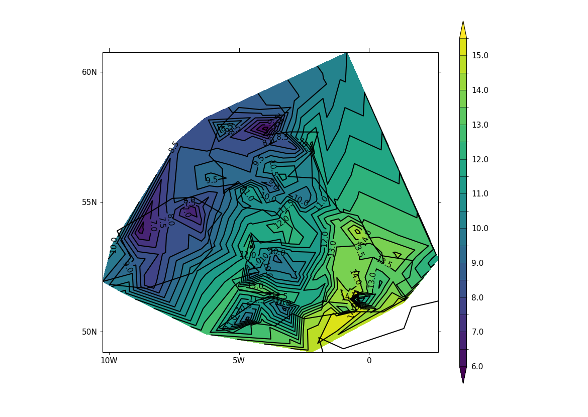
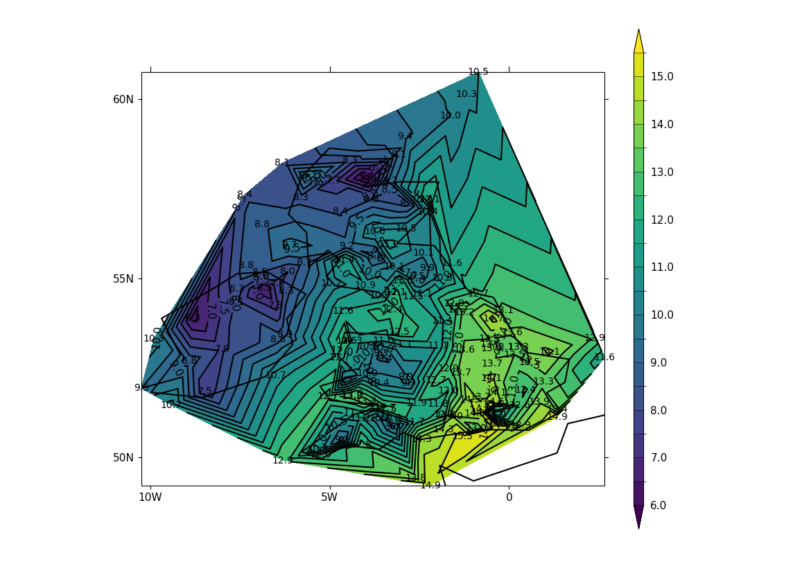
To see if this plot is correct we can add some extra code to that above to plot the station locations and values at that point, as below. The decimal point is roughly where the data point is located.

Example 26b: Contour plot from discrete feature values with labelling#

Making a contour plot where the contours are determined from discrete feature values with labels to annotate the values at each feature, in this case station data with values at each station annotated#

# Arrays for data
lons = []
lats = []
pressure = []
temp = []

# Read data and make the contour plot
f = open("cfplot_data/synop_data.txt")
lines = f.readlines()
for line in lines:
    mysplit = line.split()
    lons = np.append(lons, float(mysplit[1]))
    lats = np.append(lats, float(mysplit[2]))
    pressure = np.append(pressure, float(mysplit[3]))
    temp = np.append(temp, float(mysplit[4]))

cfp.gopen()
cfp.con(
    x=lons, y=lats, f=temp, ptype=1, colorbar_orientation="vertical"
)
for i in np.arange(len(lines)):
    cfp.plotvars.mymap.text(
        float(lons[i]),
        float(lats[i]),
        str(temp[i]),
        horizontalalignment="center",
        verticalalignment="center",
        transform=ccrs.PlateCarree(),
    )

cfp.gclose()