Trajectories

Data stored as discrete sampling geometries, such as contiguous ragged array format, can be plotted using cf-plot. Multiple trajectories represented by multidimensional-arrays with a trajectory dimension can be plotted, as below.

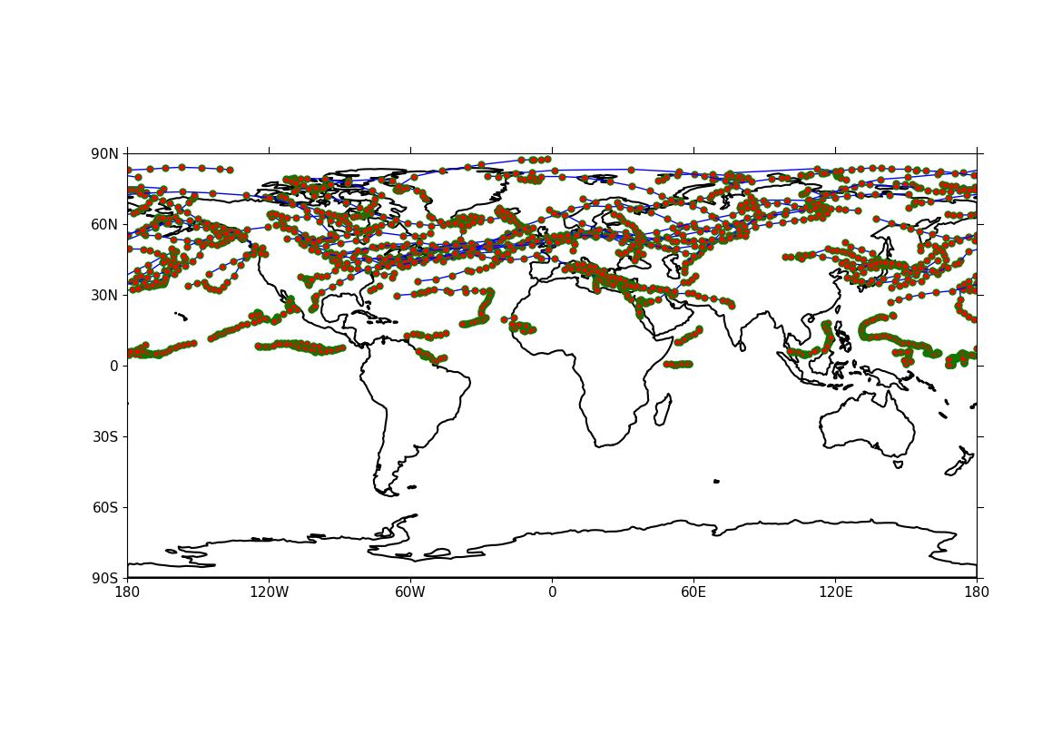
Example 39: Basic track plotting

A basic example of plotting a track i.e. trajectory

f = cf.read(f"cfplot_data/ff_trs_pos.nc")[0]

cfp.traj(f)

Single trajectories can also be plotted, including those in one-dimensional array form, as below.

Example 39b: plotting a single (1D) DSG trajectory

Plotting data for a single trajectory encoded as a discrete sampling geometry in the form of a one-dimensional array, as standard)

f = cf.read(f"cfplot_data/dsg_trajectory.nc")[0]

cfp.traj(f)

This a plot of relative vorticity tracks is made in the cylindrical projection.

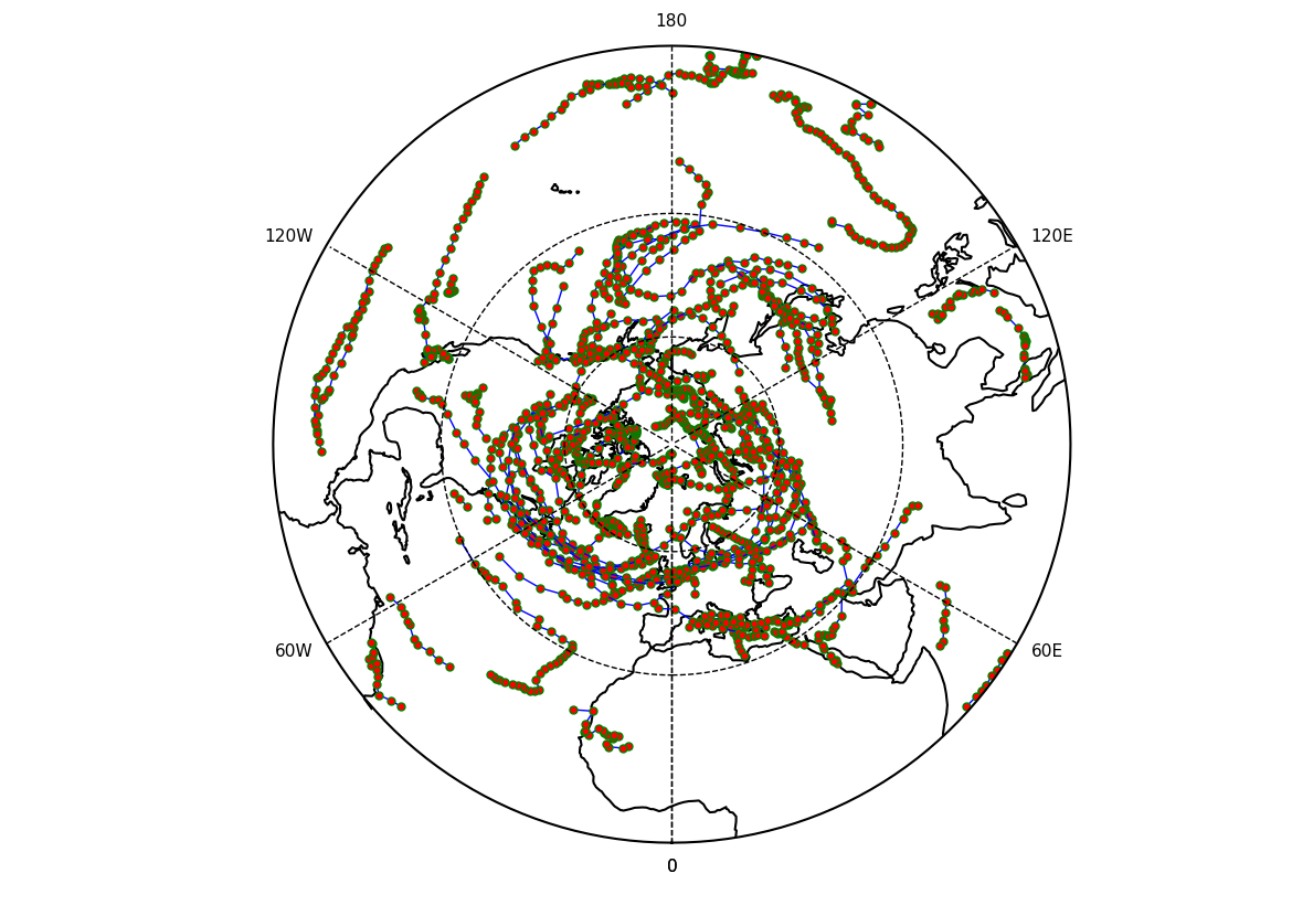
Example 40: Tracks in the polar stereographic projection

Plotting tracks i.e. trajectories on the Northern polar stereographic projection

f = cf.read(f"cfplot_data/ff_trs_pos.nc")[0]

cfp.mapset(proj="npstere")

cfp.traj(f)

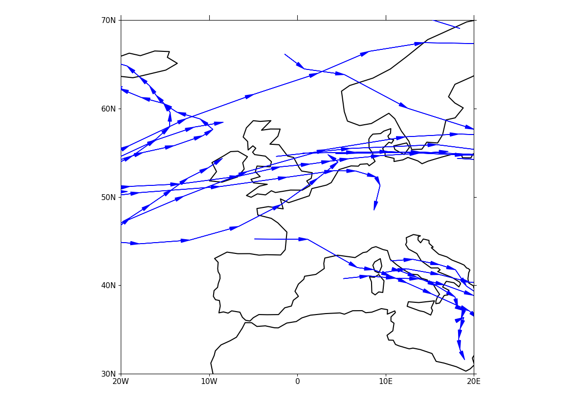
Example 41: Feature propagation over Europe

Plotting the propagation of features over Europe

f = cf.read(f"cfplot_data/ff_trs_pos.nc")[0]

cfp.mapset(lonmin=-20, lonmax=20, latmin=30, latmax=70)

cfp.traj(f, vector=True, markersize=0.0, fc="b", ec="b")

Example 42a: Tracks with labelled data points

Plotting tracks with labelling of the discrete data points forming the trajectory shown with intensity matched to a displayed colour scale using the legend keyword

f = cf.read(f"cfplot_data/ff_trs_pos.nc")[0]

cfp.mapset(lonmin=-50, lonmax=50, latmin=20, latmax=80)
g = f.subspace(time=cf.wi(cf.dt("1979-12-01"), cf.dt("1979-12-10")))
g = g * 1e5
cfp.levs(0, 12, 1, extend="max")
cfp.cscale("scale1", below=0, above=13)

cfp.traj(
    g,
    legend=True,
    markersize=40.0,
    colorbar_title="Relative Vorticity (Hz) * 1e5",
)

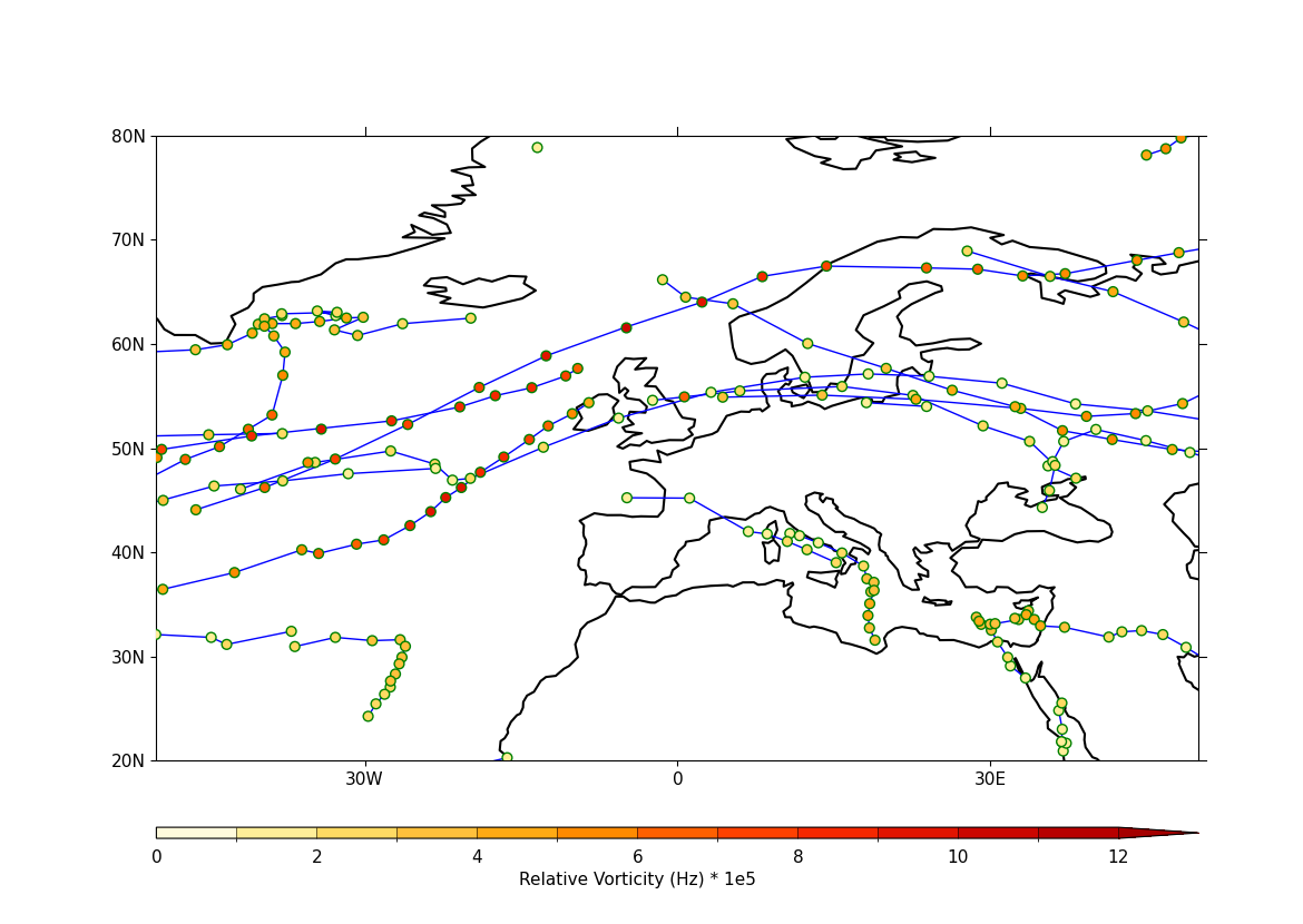
In this plot the tracks between 1979-12-01 and 1979-12-30 are selected and labelled according intensity with a colour bar.

Example 42b: Tracks displayed in a colour scale

Plotting tracks where the trajectory is shown in colours mapped to a colour scale corresponding to the value of the underlying data by setting the legend_lines keyword to True

f = cf.read(f"cfplot_data/ff_trs_pos.nc")[0]

cfp.mapset(lonmin=-50, lonmax=50, latmin=20, latmax=80)
g = f.subspace(time=cf.wi(cf.dt("1979-12-01"), cf.dt("1979-12-10")))
g = g * 1e5
cfp.levs(0, 12, 1, extend="max")
cfp.cscale("scale1", below=0, above=13)
cfp.traj(
    g,
    legend_lines=True,
    linewidth=2,
    colorbar_title="Relative Vorticity (Hz) * 1e5",
)

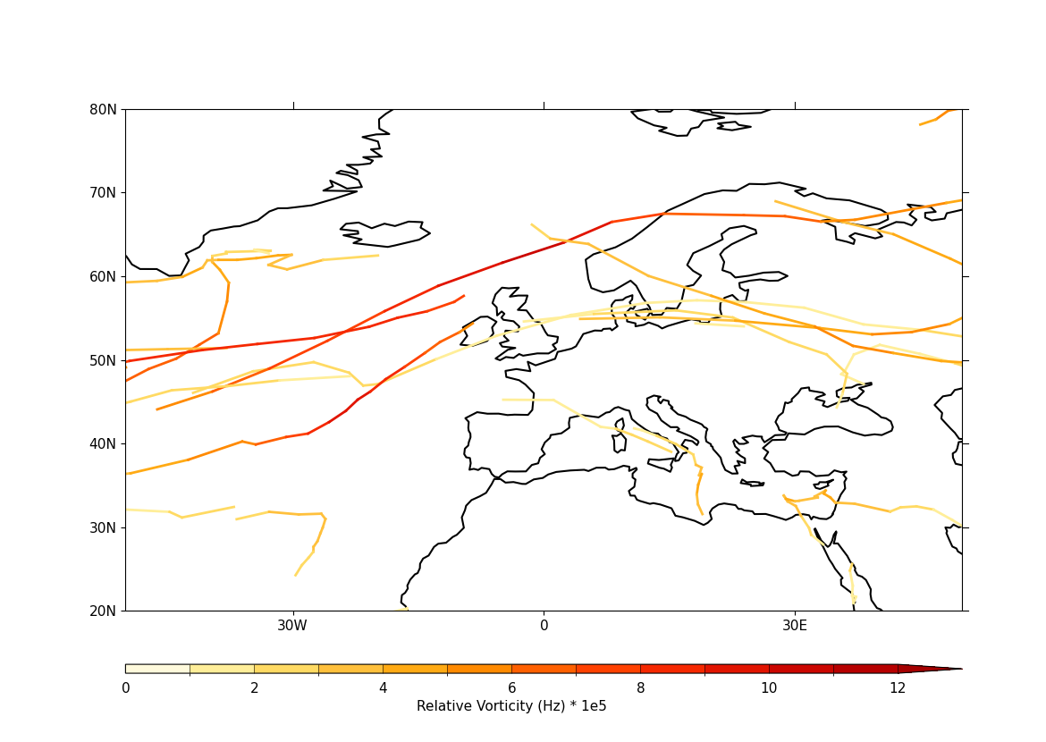
Selecting legend_lines=True plots lines only and colours them according to the sum of the start and end point divided by two. This can be a useful option when there are lots of trajectories.